
Last time, we have seen that every arc chain is an arc. This month, we will see that every arc is an arc chain. Let me recall some definitions first.
An arc is a compact, connected Hausdorff space with exactly two non-cut-points.
An arc chain is a compact, connected topological space X of cardinality at least 2, with a semiclosed total ordering ≤. By semiclosed, we mean that the downward closure and the upward closure of any point is closed.
We have seen that every arc chain is a complete lattice in its ordering ≤, hence it has a least element ⊥ and a largest element ⊤; then, this arc chain is an arc, with ⊥ and ⊤ as its sole non-cut-points. We have also seen that arc chains can be characterized entirely order-theoretically: they are exactly the order-dense, non-trivial pointed d-chains, and their topology is the patch (or Lawson) topology of their Scott topology, and is generated by open and half-open intervals—which I called o-intervals (see Proposition D of last time).
We will see that every arc can be equipped with a total ordering that turns it into an arc chain. Before we do so, we will see that this is somewhat surprising, because every arc chain is locally connected, but there does not seem to be any reason why arcs should be. Of course, in the end, this means that every arc really is locally connected. But this will take several steps.
Local connectedness
A topological space is locally connected if and only if for every point x, for every open neighborhood U of x, there is connected open neighborhood V of x included in U.
Let me recall the following notion from last time. An o-interval in an arc chain (X, ≤) is an open interval ]a, b[ with a<b (the set of all points strictly between a and b), or a half-open interval [⊥, b[ with ⊥<b or ]a, ⊤] with a<⊤.
Proposition A. Every o-interval in an arc chain is connected. Therefore every arc chain is locally connected.
Proof. Let (X, ≤) be an arc chain.
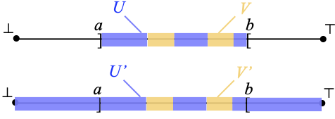
We first show that an open interval ]a, b[, with a<b, is connected. Otherwise, there are two open subsets U and V of X such that U ⋂ ]a, b[ and V ⋂ ]a, b[ are non-empty, disjoint, and such that ]a, b[ ⊆ U ∪ V. Replacing U by U ⋂ ]a, b[ and V by V ⋂ ]a, b[ if necessary, and noting that those intersections are still open, we obtain a partition of ]a, b[ as U ∪ V for two non-empty disjoint open subsets of X. Look at the following picture, where I have drawn U in blueberry blue and V in orange.

By Proposition D of last time, U is the union of a family F of pairwise disjoint o-intervals, and because neither ⊥ nor ⊤ is in U, those intervals are all open intervals ]a’, b’[. At most one can be such that a’=a, and at most one can be such that b’=b, because those intervals are non-empty and disjoint. Additionally, none can be such that both a’=a and b’=b: for example, if U contained an interval ]a’, b’[ with a’=a and b’=b, then U would contain ]a, b[, forcing V to be empty, which is impossible. We reason similarly with V, expressing it as the union of a family G of pairwise disjoint open intervals. It follows that among the intervals in F ∪ G, exactly one has a as its left end-point (call it I) and exactly one has b as its right end-point (call it J). In the picture above, I is the leftmost blueberry blue region, and J is the rightmost orange region.
Let us write I as ]a, b’[ and J as ]a’, b[. We define I’ ≝ [⊥, b’[ and J’ ≝ ]a’, ⊤]. Replacing I by I’ and J by J’, we will form a partition of X in two disjoint non-empty open subsets U’ and V’. For example, in the situation pictured above, U’ and V’ are as shown below.
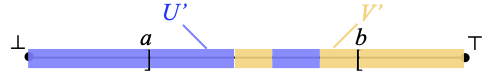
In general, there are four cases to consider, according to whether a is blue or orange, and according to whether b is blue or orange. Explicitly:
- if I is in F and J is in G, then we let U’ be the union of all the intervals in F, except for I which we replace by I’, and V’ be the union of all the intervals in G, except for J which we replace by J’ (this is the case that I have illustrated above);
- the case where I is in G and J is in F is symmetric: U’ is the union of all the intervals in F, except for J which we replace by J’, and V’ is the union of all the intervals in G, except for I which we replace by I’;
- if both I and J are in F, then we let U’ be the union of all the intervals in F, except for I which we replace by I’ and for J which we replace by J’, and V’ ≝ V; the situation is shown below:
- the case where both I and J are in G is symmetric: V’ is the union of all the intervals in G, except for I which we replace by I’ and for J which we replace by J’, and U’ ≝ U.
I hope it is easy to see that, in each case, U’ and V’ are disjoint open subsets of X, and that their union is the whole of X. Additionally, U’ contains U and V’ contains V, so they are both non-empty. Hence U’ and V’ form a partition of X in two disjoint non-empty open sets. That is impossible since X is connected, by definition of arc chains. Therefore ]a, b[ is connected.
The proof that o-intervals [⊥, b[ or ]a, ⊤] are connected is similar, but simpler. Let us deal with [⊥, b[; the other case is symmetric. We assume that [⊥, b[ is not connected, and therefore we can write it as U ∪ V for two non-empty disjoint open subsets of X. We define F and G from U and V respectively, as above. There is exactly one interval I in F ∪ G that contains ⊥, and there is exactly one (necessarily disjoint) interval J in F ∪ G whose right end-point is b. Writing J as ]a’, b[ (it cannot be of another form), we define J’ ≝ ]a’, ⊤]. There is no need to define a replacement I’ for I. We define U’ and V’ as follows:
- if J is in F, then we define U’ as the union of all the intervals in F, except for J which we replace by J’, and we let V’ ≝ V;
- if J is in G, then we define V’ as the union of all the intervals in G, except for J which we replace by J’, and we let U’ ≝ U.
Then U’ and V’ define a partition of X in two disjoint non-empty open subsets of X, which is impossible. Therefore [⊥, b[ is connected.
We can now conclude that X is locally connected. Let x ∈ X and let U be an open neighborhood of x in X. By Proposition D of last time, U contains an o-interval I that contains x. We have just shown that I is connected. ☐
Separation
In order to prepare the grounds for showing that we can turn any arc into an arc chain, we need to talk about separation.
Two subsets A and B of a topological space are separated if and only if the closure of A is disjoint from B and the closure of B is disjoint from A. Two separated subsets are disjoint, but, for example, [0, 1] and ]1, 2] are disjoint but not separated in R.
We write A|B to say that A and B are separated and non-empty.
We recall that a space is connected if and only if it cannot be written as the union of two disjoint non-empty open subsets. By trading those open subsets with their complements, we see that a space is connected if and only if it cannot be written as the union of two disjoint non-empty closed subsets.
Lemma B. A space X is connected if and only if one cannot write X as A ∪ B with A|B.
Proof. If X = A ∪ B where A|B, then A ⊆ cl(A) ⊆ X–B (since A and B are separated) ⊆ A (since X = A ∪ B), so A = cl(A) and therefore A is closed. Similarly, B is closed. Since A and B are separated, they are disjoint, and since X = A ∪ B, they form a partition of X. Each of them is closed and non-empty, so X is not connected.
Conversely, if X is not connected, then we can write X as the union of two disjoint non-empty open subsets U and V. Then U is included in the closed set X–V, hence cl(U) is also included in X–V, so cl(U) and V are disjoint; similarly, cl(V) and U are disjoint, so U|V. ☐
We recall that a cut-point of X is a point x of X such that X–{x}, as a subspace, is not connected. The following lemma serves to be able to talk about cut-points without having to get involved with subspaces.
Lemma C. Let X be a connected T1 space. A point x of X is a cut-point of X if and only if there are two non-empty separated subsets A and B of X such that A ∪ B = X–{x}.
Proof. If x is a cut-point of X, then X–{x} is not connected, so we can write X–{x} as the union U ∪ V of two disjoint non-empty subsets of X–{x}. Since X is T1, X–{x} is itself open in X, so U and V are open in X, not just in X–{x}. Let us write cl(_) for closure in X (not in X–{x}). Since U is disjoint from V, it is included in the complement X–V, which is closed in X, so cl(U) ⊆ X–V, and therefore cl(U) and V are disjoint. Symmetrically, cl(V) and U are disjoint. Therefore U|V, and we can take A ≝ U, B ≝ V.
Conversely, let A|B and let us assume that A ∪ B = X–{x}. Since A and B are separated, cl(A) is included in X–B, so cl(A) ⋂ (X–{x}) ⊆ X–B–{x} = A. The reverse inclusion A ⊆ cl(A) ⋂ (X–{x}) is clear, so A = cl(A) ⋂ (X–{x}), showing that A is closed in the subspace X–{x}. Similarly, B is closed in X–{x}. They are disjoint and their union is X–{x}, so the complement of A in X–{x} is B, showing that A is not just closed but also open in X–{x}; similarly for B. We have found two open subsets, A and B, of X–{x}, which are non-empty, disjoint, and whose union is X–{x}. Therefore x is a cut-point of X. ☐
The sets A and B involved in Lemma C cannot be completely arbitrary. Here is why.
Lemma D. Let X be a connected T1 space, and x be a cut-point of X. Let X–{x} be written as A ∪ B where A|B. Then A ∪ {x} and B ∪ {x} are connected, closed, and A and B are open in X.
Proof. Writing cl(_) for closure in X, the fact that A|B implies that cl(B) is disjoint from A, hence is included in B ∪ {x}. Therefore cl(B) is equal to B or to B ∪ {x}. In the second case, B ∪ {x} is equal to cl(B), and in the first case, it is equal to cl(B) ∪ {x}. In both cases, B ∪ {x} is closed in X: {x} is closed because X is T1. Since A is the complement of B ∪ {x} in X, A is open in X.
Similarly, A ∪ {x} is closed, and B is open in X.
Let us assume that A ∪ {x} is not connected; the case of B ∪ {x} is similar. We can write A ∪ {x} as the union of two disjoint non-empty closed subsets of A ∪ {x}, seen as a subspace of X. Since A ∪ {x} is closed in X, its closed subsets are just the closed subsets of X that are included in A ∪ {x}: every closed subset of A ∪ {x} is of the form C ⋂ (A ∪ {x}) where C is closed in X, and then C ⋂ (A ∪ {x}) is also closed in X, and included in A ∪ {x}. Hence we can write A ∪ {x} as the union of two disjoint, non-empty closed subsets C and D of X. Up to symmetry, we assume that x is in D, and therefore not in C. Then X is the union of C and of D ∪ (B ∪ {x}), which are both closed. Since x ∈ D, D ∪ (B ∪ {x}) = D ∪ B, and we then see that C and D ∪ B are disjoint: no point of C can be in D, since C and D are disjoint, and no point of C, which is included in A ∪ {x}, can be in B. Also, C and D ∪ B are non-empty. This is impossible since X is connected. ☐
It is not the case in general that A itself, or B, is connected. For example let X be a plus sign shape inside the space R2, namely the subspace of points {0} × [-1, 1] union [-1, 1] × {0}.
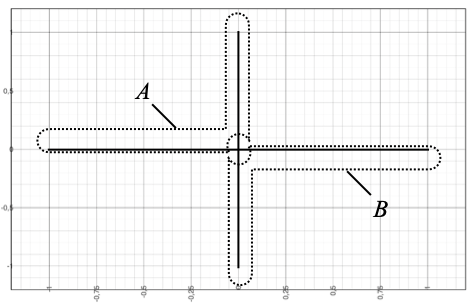
The origin (0, 0) is a cut-point, and we can write X–{(0, 0)} as A ∪ B where A|B by letting A consist of the union of the two rays {0} × ]0, 1] and [-1, 0[ × {0}, and B consist of the union of the two remaining rays {0} × [-1, 0[ and ]0, 1] × {0}; none of A and B is connected.
The cut-point ordering
Separation leads us to the following definition.
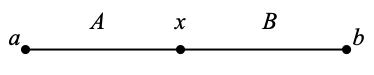
Definition. In a connected space X, given three points a, x, and b, we say that x separates a and b, in notation [a, x, b] if and only if one can write X–{x} as A ∪ B where A|B, a ∈ A and b ∈ B.
Given a point e of X, the binary relation ≤e is defined on X by x ≤e y if and only if x=e, or x=y, or [e, x, y].
This definition of the cut-point ordering ≤e—yes, we will see that it is a partial ordering—can be found, say, in L. E. Ward [1, Section 3]. I am not saying he was the first to define it, though.
By Lemma C, [a, x, b] entails that x must be a cut-point of X. The rough idea is that X has the following shape: if you want to go, continuously, from a to b, then you will have to go through x.
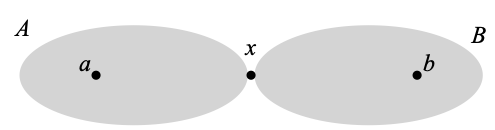
This picture may give you the wrong impression that A and B are connected. We have just seen (Lemma D) that A ∪ {x} and B ∪ {x} are connected, but A and B may fail to be.
If X is an arc, then it has exactly two non-cut-points. If a and b are these two non-cut-points, all the remaining points are cut-points, and the shapes A and B above should really look as follows:
A lot of what we have proved and of what we will prove holds on arbitrary connected T1 spaces. Even on a compact, connected, Hausdorff space (in short, on a continuum), the notions of separation [a, x, b] and the relation ≤e—which will turn out to be a partial ordering with pretty special properties—make sense.
It makes sense, but it may be pretty trivial.
Example 1. If X is a circle, then it has no cut-point whatsoever. Hence [e, x, y] is always false, and therefore x ≤e y if and only if x=e or x=y, for all points x and y in this space. In other words, ≤e makes every pair of points incomparable, except for e, which is placed below all other points.
Example 2. The following infinity shape is an example of a continuum with exactly one cut-point, shown as e below.
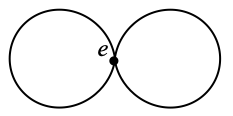
Since there is no other cut-point, as in Example 1, [e, x, y] is always false, and ≤e makes every pair of points incomparable, except for e, which is placed below all other points.
Example 3. We take the same infinity shape, but we take e to be any non-cut-point instead (see below).
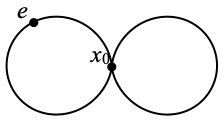
Since [e, x, y] implies that x is a cut-point, and there is only one—the point x0 above—, [e, x, y] implies x=x0. The only way we can write X–{x0} as A ∪ B where A|B and e ∈ A is by taking for A the left circle minus x0, and for B the right circle minus x0; indeed, by Lemma D, A ∪ {x0} and B ∪ {x0} have to be connected. Therefore [e, x, y] if and only if x=x0 and y is in that set B. As a consequence, ≤e is characterized as follows: e is at the bottom, right above we find x0 and the points of the left circle A, all pairwise incomparable, and then all the remaining elements, from B, are pairwise incomparable and placed above x0.
We will use the following several times.
Lemma E. Let X be a connected space.
- If Ai|Bi in X, for every i in an arbitrary non-empty set I, and if ∩i ∈ I Ai is non-empty, then ∩i ∈ I Ai | ∪i ∈ I Bi.
- If A|B and C|D in X, and if A intersects C, then (A ⋂ C) | (B ∪ D).
Proof. 1. We have ∩i ∈ I Ai ≠ ∅ by assumption. Since I is non-empty and each Bi is non-empty, ∪i ∈ I Bi is non-empty, too. The closure of ∪i ∈ I Bi is equal to ∪i ∈ I cl (Bi), and since each set cl (Bi) is disjoint from Ai, hence from the smaller set ∩i ∈ I Ai, cl (∪i ∈ I Bi) is also disjoint from ∩i ∈ I Ai. The closure of ∩i ∈ I Ai is included in cl (Ai) for every i in I, and cl (Ai) is disjoint from Bi, so cl (∩i ∈ I Ai) is disjoint from Bi for every i in I. Therefore it is also disjoint from ∪i ∈ I Bi.
2. follows from 1 by taking a two element indexing set for I. ☐
≤e is a partial ordering
Proposition F below is basically Proposition 3 of Ward’s paper [1], except that we do not require e to be a cut-point—this will be needed, as I plan to use the following lemma precisely when e is a non-cut-point—and the assumptions I am making are less restrictive than Ward’s.
Proposition F. Given any point e of a connected T1 space X, ≤e is a partial ordering on X, whose least element is e.
Proof. It is clearly reflexive, and we have e ≤e x for every x in X by definition, so e is least. As far as antisymmetry and transitivity are concerned, we will need to show the following first.
- (*) For any two points x and y, [e, x, y] and [e, y, x] cannot hold at the same time.
Indeed, let us assume that [e, x, y] and [e, y, x].
By definition, we can write X–{x} as A ∪ B where A|B, e ∈ A and y ∈ B, and we can write X–{y} as C ∪ D where C|D, e ∈ C and x ∈ D. We note in particular that any of those two statements implies x≠y.
Since A and C intersect (at e), we can use Lemma E, item 2, and we obtain that (A ⋂ C) | (B ∪ D).
We can write X as the union of A ⋂ C and of B ∪ D. Indeed, (A ⋂ C) ∪ (B ∪ D) = (A ∪ B ∪ D) ⋂ (C ∪ B ∪ D), A ∪ B ∪ D = (X–{x}) ∪ D = X (since x ∈ D), C ∪ B ∪ D = B ∪ (X–{y}) = X (since y ∈ B), so (A ⋂ C) ∪ (B ∪ D) = X.
Hence X = (A ⋂ C) ∪ (B ∪ D) with (A ⋂ C) | (B ∪ D). But this is impossible by Lemma B, since X is connected. - (**) For every point x, [e, x, e] is false. Indeed, [e, x, e] means that we can write X–{x} as A ∪ B where A|B, e ∈ A and e ∈ B. But since A|B, A and B are disjoint, and therefore cannot both contain e.
We can now show that ≤e is antisymmetric. Let us assume that x ≤e y and y ≤e x, but that x≠y. By (*), it is impossible that [e, x, y] and [e, y, x], so either x=e and [e, y, x], or [e, x, y] and y=e. In other words, [e, y, e] or [e, x, e], and both are impossible by (**).
In order to show transitivity, we claim that: (***) for any three points x, y and z, if [e, x, y] and [e, y, z] then [e, x, z].
In order to show this, let us assume that [e, x, y] holds, so we can write X–{x} as A ∪ B where A|B, e ∈ A and y ∈ B; and let [e, y, z] hold, so we can write X–{y} as C ∪ D where C|D, e ∈ C and z ∈ D.
We cannot have x ∈ D. Indeed, if x ∈ D then X–{y} = C ∪ D where C|D, e ∈ C and x ∈ D, so [e, y, x]; but we also have [e, x, y], and this is ruled out by (*). Having shown x ∉ D, it follows that (X–{x}) ∪ D = X–{x}. Since y ∈ B, we have B ∪ (X–{y}) = X.
Now (A ⋂ C) ∪ (B ∪ D) = (A ∪ B ∪ D) ⋂ (C ∪ B ∪ D) = ((X–{x}) ∪ D) ⋂ (B ∪ (X–{y})) = (X–{x}) ⋂ X = X–{x}. Since e is both in A and in C, we can apply Lemma E, item 2, and therefore (A ⋂ C) | (B ∪ D). Since z ∈ D ⊆ B ∪ D, this shows that [e, x, z], proving (***).
Now let x ≤e y and y ≤e z. If x=y or if y=z, it is immediate that x ≤e z. Similarly if x=e, since e is least in ≤e. Let us now assume that x≠y, y≠z, and x≠e. In particular, x ≤e y means [e, x, y]. It is then impossible that y=e, by (**). Since y≠z and y≠e, the fact that y ≤e z then means [e, y, z]. Then [e, x, z] by (***), whence x ≤e z. ☐
≤e is tree-like
Let us write ↑e and ↓e for upward closure and downward closure (respectively) with respect to ≤e. The following says that X is tree-like: a tree is a well-founded partially ordered set (where x≤y means “x lies on the branch from the root to y“) with a unique least element e (the root), and such that the downward closure of every point is totally ordered. By tree-like, we mean the same notion, without the requirement of well-foundedness. Here is a view of the situation, where going up with respect to ≤e means going right:
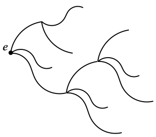
This picture is deceptively simple, though: there are only finitely many branches, and the space (if embedded in the plane) is compact, notably.
Lemma G. Let X be a connected T1 space and e ∈ X. For every x ∈ X, ↓e x is totally ordered by ≤e.
Proof. The proof is similar to that of Proposition 6 of [1].
Let y and z be two points of X that lie in ↓e x. We must show that one of them is less than or equal to the other one. If y=e, then y ≤e z, since e is the least element with respect to ≤e, by Proposition F; similarly if z=e. If y=x, then z ≤e x=y, and similarly y ≤e z if z=x. Henceforth, we will assume that y and z are both distinct from e, and both distinct from x.
Since y ≤e x and y≠x, y≠e, we must have [e, y, x]. Therefore we can write X–{y} as A ∪ B where A|B, e ∈ B and x ∈ A. (Yes, we are swapping the roles of A and B; this will allow us to use Lemma E, item 2, without having to change the names of the various sets involved.) Similarly, since z ≤e x and z≠x, z≠e, we must have [e, z, x], so we can write X–{z} as C ∪ D where C|D, e ∈ D and x ∈ C.
Let us assume that y ≰e z. Then y≠z, and it is not the case that [e, y, z], so z cannot be in A: if z were in A, we would have [e, y, z] since A|B and e ∈ B. Therefore z ∈ B. A and C intersect (at x), so (A ⋂ C) | (B ∪ D) by Lemma E, item 2. The union (A ⋂ C) ∪ (B ∪ D) is equal to (A ∪ B ∪ D) ⋂ (C ∪ B ∪ D) = ((X–{y}) ∪ D) ⋂ (B ∪ (X–{z})). Since z ∈ B, B ∪ (X–{z}) = X. If y were in D, then (X–{y}) ∪ D would be equal to X, so we would have (A ⋂ C) ∪ (B ∪ D) = X, with (A ⋂ C) | (B ∪ D). This is impossible since X is connected, using Lemma B. Therefore y ∉ D. Since y≠z, y is in C. This entails [e, z, y], hence z ≤e y. ☐
Is ≤e semiclosed?
Let us investigate whether ≤e is semiclosed. A semiclosed ordering is one that is upper semiclosed (↑e x is closed for every point x) and lower semiclosed (↓e x is closed for every point x).
Lemma H. Let X be a connected T1 space and e ∈ X.
- The ordering ≤e is upper semiclosed: for every x ∈ X, ↑e x is closed in X.
- For every x ∈ X, the set of points strictly larger than x with respect to ≤e is open in X.
- For every z ∈ X, for every x ≤e z, ↓e x is closed in the subspace ↓e z of X.
Proof. 1. If x=e, then ↑e x = X, since e is the least element with respect to ≤e, by Proposition F. Henceforth, let us assume x≠e.
The elements of ↑e x are the points y such that y=x or [e, x, y], namely they are the elements of {x} ∪ {y ∈ X | ∃ A, B with A|B, A ∪ B = X–{x}, e ∈ A, y ∈ B}. Hence ↑e x is the union of {x} with ∪A, B B, where the latter union ranges over all pairs of subsets A and B of X such that A|B, A ∪ B = X–{x} and e ∈ A. In what remains of this proof, I will keep the same convention, and I will write ∪A, B B instead of writing ∪A, B with A|B, A ∪ B = X–{x}, e ∈ A B, which would be heavy; I will do the same with intersections.
If there is no such pair of subsets A and B, then ↑e x is just {x}, which is closed since X is T1. Otherwise:
- We use Lemma E, item 1, on the (now non-empty) family of pairs A, B such that A|B, A ∪ B = X–{x} and e ∈ A, and we obtain that ∩A, B A | ∪A, B B. We can, because ∩A, B A contains e, and is therefore non-empty.
- We claim that the union of ∩A, B A with ∪A, B B is equal to X–{x}. For every point y in X–{x}, if y is not in ∩A, B A, then there is a pair A, B as above such that y is not in A; since y≠x, y must be in B. Conversely, every point of ∩A, B A is in some A of one of those pairs of subsets A, B (because there is such a pair of subsets A, B), hence is different from x; and every point of ∪A, B B is in some B of one of those pairs of subsets A, B, hence is different from x.
- This allows us to use Lemma D on the pair ∩A, B A, ∪A, B B, and conclude that (∪A, B B) ∪ {x} is closed in X. But this is just ↑e x, as we have seen near the beginning of this argument.
2. If e=x, then the points strictly larger than x are exactly all the points of X–{e}, since e is least element with respect to ≤e, by Proposition F. This is open since X is T1.
If e≠x, then the points strictly larger than x are the points y such that [e, x, y], hence are the points in ∪A, B B, where we take the same conventions as above. We have seen that ∩A, B A | ∪A, B B and that the union of ∩A, B A and of ∪A, B B is equal to X–{x}, so ∪A, B B is open by Lemma D.
3. Let us assume that x ≤e z. Let U be the set of points strictly larger than x with respect to ≤e. By item 2, U is open in X. Now ↓e z – ↓e x is the set of points y such that y ≤e z and y ≰e x. By Lemma G, ↓e z is totally ordered by ≤e, so “y ≤e z and y ≰e x” is equivalent to “y ≤e z and y is strictly larger than x”, hence ↓e z – ↓e x is equal to ↓e z ⋂ U. Then, ↓e x = ↓e z – (↓e z – ↓e x): by Boolean reasoning, ↓e z – (↓e z – ↓e x) = ↓e z ⋂ ↓e x, and that is equal to ↓e x since x ≤e z. Therefore ↓e x = ↓e z – (↓e z ⋂ U) = ↓e z – U. Since U is open, ↓e x is closed in the subspace ↓e z. ☐
Lemma H is somewhat frustrating: ↑e x is closed is closed in X, but it does not tell us whether ↓e x is also closed in X, only in all its subspaces of the form ↓e z, where x ≤e z. Now, we have not yet used any compactness assumption on X, and it is time to do so.
Compact, connected T1 spaces are arc-chains
Lemma I. Let X be a compact, connected T1 space and e ∈ X. For every x ∈ X, there is a maximal point above x with respect to ≤e. If X contains at least two elements, this maximal point is a non-cut-point.
Proof. For the first part, we use Zorn’s Lemma, and we show that (X, ≤e) is inductive. Let C be a totally ordered, non-empty subset of (X, ≤e). The set of upper bounds of C is the intersection of the sets ↑e y where y ranges over C. By Lemma H, item 1, those are all closed. Hence (↑e y)y ∈ C is a filtered family (even a chain) of non-empty closed subsets of the space X. Since X is compact, this intersection is non-empty (see Proposition 4.4.9 in the book, for example), and any element of this intersection is an upper bound of C.
For the second part, let y be a maximal point of (X, ≤e), and let us assume that X contains at least two points. This entails that y≠e: otherwise there would be no point strictly above the least element e in (X, ≤e), so e would be the sole element of X. If y is a cut-point, then by Lemma C, there are two non-empty separated subsets A and B of X such that A ∪ B = X–{y}. Since y≠e, e is in A or in B; by symmetry, we may assume that e is in A. But B is non-empty. We pick a point z from B. Then [e, y, z], so z is strictly larger than y with respect to ≤e. This is impossible since y was chosen maximal. ☐
Remark. In a connected T1 space X with at least two elements, and picking e ∈ X, the maximal elements of (X, ≤e) are exactly its non-cut-points (except for e if e is a non-cut-point). The maximal ⇒ non-cut-point direction is really what we proved in the second half of the proof of Lemma I—we did not use compactness there. Conversely, let x be a non-cut-point of X different from e. By Lemma B, we cannot write X–{x} as A ∪ B where A|B. Hence [e, x, y] for no point y ∈ X, showing that y is maximal. I invite you to look back at Example 3 (the infinity shape with e placed on the left circle, and a single cut-point x0 at the intersection of the two circles): except for the least element e and the cut-point x0, all the other points are maximal.
We can now prove the main theorem of this post. We recall that an arc is a compact, connected Hausdorff space with exactly two non-cut-points. We only need T1-ness instead of Hausdorffness in the following, but Hausdorffness is implied, as item 4 below shows.
Theorem J (Arc ↦ arc chain). Let X be a compact, connected T1 space with exactly two non-cut-points a and b. Then:
- b is the largest element of X with respect to ≤a;
- ≤a is a semiclosed total ordering;
- (X, ≤a) is an arc chain;
- X is Hausdorff;
- X is locally connected.
Proof. 1. Let x be any point of X. By Lemma I, there is a maximal point z above x with respect to ≤a, and it is a non-cut-point. We cannot have z=a: since z is maximal, that would imply that no element is strictly larger than a with respect to ≤a, hence that X={a}; but X has two non-cut-points, hence contains at least two points. Since z≠a, since z is a cut-point, and since we have only got two, which are a and b, z must be the other one, namely z=b. Therefore x is in ↓a b.
The point x was arbitrary. Hence X = ↓a b. Equivalently, b is the largest element of X with respect to ≤a.
2. By Lemma H, item 1, ≤a is upper semiclosed. Let x be any point of X. By Lemma H, item 3, taking z ≝ b, and recalling from item 1 (which we have just proved) that x ≤a b, we obtain that ↓a x is closed in the subspace ↓a b of X. But item 1 above shows that ↓a b is in fact the whole of X. Therefore ↓a x is closed in X, for every x ∈ X: ≤a is lower semiclosed. In other words, ≤a is semiclosed.
3. An arc chain is a compact, connected topological space X of cardinality at least 2, with a semiclosed total ordering ≤. We have just showed that ≤a is semiclosed, and all the other properties are assumptions that we have made on X.
4. In Proposition C of last time, we have shown that every arc chain is a compact pospace. In particular, it is Hausdorff (Proposition 9.1.12 in the book).
5. Proposition A of this post states that every arc chain is locally connected. ☐
Remark. There are really (at least) two ways to see an arc X as an arc chain. Given its two non-cut-points a and b, we can either build (X, ≤a), where a is least and b largest, or (X, ≤b), where b is least and a alrgest. Hence the construction of an arc chain from an arc is not functorial.
Item 5 in Theorem J is perhaps surprising—unless you remember that I had announced it near the beginning of this post: every arc is locally connected, although nothing in the definition of an arc (compact, connected Hausdorff space with exactly two non-cut-points) states it clearly.
The uniqueness of second-countable arcs
We are not too far from showing a result I mentioned last time, namely that every second-countable arc is homeomorphic to [0, 1]. I said that, apparently, the result was due to Oswald Veblen, according to this post on the Math Stackexchange; however, due to a missing link, I was unable to confirm this. The intended source is perhaps Veblen’s 1905 paper [2], but I have not recognized the result in there. One can find a very closely related result in a paper by Leon W. Cohen in 1929 [3, Theorem I], which states that a subset M of a metric space is homeomorphic to a closed interval [0, 1] (with a being the image of 0 in M and b being the image of 1) if and only if it is a “compact continuum” containing a and b and whose points are all cut-points, except possibly for a and b. I guess one would just say “continuum” instead of “compact continuum” today. This is close enough: by Urysohn’s metrization theorem (Exercise 6.3.18 in the book), every second-countable T4 space is metrizable, and every continuuum, in general every compact Hausdorff space is T4 (Proposition 4.4.17 in the book). Oh, Cohen does not assume that a and b are non-cut-points, but that is not necessary: every continuum of cardinality at least 2 must have at least two non-cut-points (see Appendix—this is the topic of [1]).
We have just shown that every arc can be equipped with an ordering ≤a that makes it an arc chain. In Theorem L of last time, we have shown that the arc chains are the same thing as the order-dense non-trivial pointed d-chains, where a d-chain is a chain that is a dcpo at the same time. The topology is the patch topology of the Scott topology, and consists of (disjoint) unions of o-intervals, namely intervals of the form ]a, b[ with a<b, or [⊥, b[, with b≠⊥, or ]a, ⊤] with a≠⊤, where ⊥ is the least element and ⊤ is the largest element of the pointed d-chain.
We have also seen that d-chains are continuous dcpos. An ω-continuous poset is a continuous poset with a countable basis, and Lemma 7.7.13 in the book states that a continuous poset is ω-continuous if and only if it is second-countable in its Scott topology. The following deals with the patch topology of the Scott topology.
Lemma K. Let P be continuous poset. The following are equivalent:
- (Pσ)patch is second-countable;
- Pσ is second-countable;
- P is ω-continuous.
Proof. We have just argued for 3⇔2. By Exercise 9.1.42 in the book, every ω-continuous poset is second-countable in its Lawson topology. By Exercise 9.1.36 in the book, for a continuous poset, the Lawson topology coincides with the patch topology (of its Scott topology). Hence 3⇒1. It remains to show the 1⇒2 direction.
Let (On)n ∈ N be a countable base of the topology of (Pσ)patch. The usual base of (Pσ)patch consists of finite intersections of open subsets and of complements of compact saturated subsets of Pσ. Since finite intersections of open subsets are open and finite unions of compact saturated subsets are compact saturated, this usual base consists of differences U–Q where U is open in Pσ and Q is compact saturated in Pσ.
Let us say that a pair of natural numbers m and n is good if and only if Om ⊆ ↟y for some point y ∈ On. For each such good pair, we pick a point y ∈ On such that Om ⊆ ↟y, and we call it ymn. (This requires a weak form of the Axiom of Choice, called the axiom of countable choice.) We note that we have picked countably many open points ymn in this way, and we claim that the sets ↟ymn form a base of the Scott topology on P, when (m, n) ranges over the good pairs.
Let x be any point of P, and V be any open neighborhood of x in Pσ. V is also open in (Pσ)patch, so by definition of the family (On)n ∈ N as a base of the patch topology, there is an n ∈ N such that x ∈ On ⊆ V. Using what we have called the usual base of Xpatch, there are an open subset U and a compact saturated subsets Q of Pσ such that x ∈ U–Q ⊆ On ⊆ V. Since P is a continuous poset, there is point y ∈ U such that x ∈ ↟y (Theorem 5.1.17 in the book). Since x ∈ ↟y, we have y ≪ x, hence y≤x, and therefore y is not in Q: since Q is upwards-closed, if y were in Q, so would be x. Hence y is in U–Q, and therefore in On.
Once again relying on the fact that (On)n ∈ N is a base of the patch topology, and since ↟y is Scott-open, there is an m ∈ N such that x ∈ Om ⊆ ↟y. Combined with the fact that y ∈ On, we realize that (m, n) is a good pair. Hence we can replace y by ymn: Om ⊆ ↟ymn, and ymn ∈ On. It follows that x ∈ Om ⊆↟ymn, and since ymn ∈ On ⊆ V and V is upwards-closed, ↟ymn ⊆ V. In short, x ∈ ↟ymn ⊆ V, proving the claim that the sets ↟ymn form a base of the Scott topology on P, when (m, n) ranges over the good pairs. ☐
Lemma K is probably not specific to continuous posets, and I have a feeling that the equivalence between a space X being second-countable and its patch space Xpatch being second-countable should extend to quasi-continuous posets and locally finitary compact spaces, with essentially the same proof. I am not sure whether it can be generalized further, but I did not really care to investigate the question any further.
The point we are interested is the following corollary of Lemma K, together with the preceding discussion.
Corollary L. The second-countable arc chains (X, ≤) are the same thing as the order-dense non-trivial pointed d-chains with a countable basis. The topology of X consists of disjoint unions of o-intervals, and coincides with the patch topology of the Scott topology of the pointed d-chain.
Now, take a second-countable arc chain, extract a countable basis, and remove the least element ⊥ and the largest element ⊤. What we obtain is a countable, order-dense subset without endpoints, namely without least or largest element.
We now observe the following well-known theorem, due to Georg Cantor.
Proposition M. Any two countable order-dense chains without endpoints are order-isomorphic.
That may sound easy. Given two order-dense posets P and Q with the same cardinality, by definition there is a bijection f of P onto Q. But there is no reason to believe that f would be monotonic, or that its inverse would be monotonic: f itself cannot in general serve as the order-isomorphism. The proof uses the back-and-forth method, a technique that Felix Hausdorff refined from Georg Cantor’s original proof, and which then came to be used extensively in model theory, a branch of logic, in the twentieth century.
Proof. We enumerate the elements of the first of the two order-dense chains without endpoints, A, as (an)n ∈ N, and the elements of the second one, B, as (bn)n ∈ N. Let us write < for the strict ordering on each of the two chains. Let us call a partial isomorphism any order isomorphism between subsets of A and B. By induction on n, we build partial isomorphisms gn between finite subsets of A and B, in such a way that a0, a1, …, an are all in the domain of gn and b0, b1, …, bn are all in the codomain of gn. When n=0, this is easy: we define g0 as mapping a0 to b0, and to be undefined on all other points. Assuming that gn has been built, we build gn+1 as follows. This will involve buiding a new partial isomorphism g’n that extends gn and whose domain contains a0, a1, …, an and an+1 as well (forth), and then we will extend g’n to the partial isomorphism gn+1 (back).
- If an+1 is already in the domain of gn, then we let g’n ≝ gn. Otherwise, we look at the position of an+1 relative to the elements in the domain of gn. Those elements form a finite chain C containing a0, a1, …, an, and an+1 is not in C.
- If an+1 is strictly larger than all the elements of C, then we pick an element b in B that is strictly larger than all elements of the image gn[C]. This is possible because B has no endpoints. We then define g’n as mapping an+1 to b—and every element x of C to gn(x).
- If an+1 is strictly smaller than all then elements of C, then symmetrically, we pick an element b in B that is strictly smaller than all elements of the image gn[C]. This is possible because B has no endpoints. We then define g’n as mapping an+1 to b, and every element x of C to gn(x).
- The interesting case is when none of the latter two cases happen. There is a largest element a of C strictly smaller than an+1, and there is a smallest element a’ of C strictly larger than an+1. Notably, a<an+1<a’. Since B is order-dense, there is an element b of B such that gn(a)<b<gn(a’). We define g’n as mapping an+1 to b, and every element x of C to g(x).
- It is easy to see that g’n is, as promised, a partial order-isomorphism that extends gn and whose domain contains a0, a1, …, an and an+1. By switching the roles of A and B, and using the same procedure, we can then extend g’n to a partial order-isomorphism gn+1 whose codomain contains b0, b1, …, bn and bn+1.
Given two partial isomorphisms g and g’, let g ⪯ g’ if and only if g’ extends g, namely if and only if the graph of g is included in the graph of g’. The poset of all partial isomorphisms (between A and B) is a dcpo, and directed suprema are obtained as unions of the graphs of the partial isomorphisms. Let g be the supremum of (gn)n ∈ N in this dcpo. Its domain contains the domain of every gn, in particular a0, a1, …, an, and similarly, its codomain contains b0, b1, …, bn for every n ∈ N. Hence g is a bijection of A onto B. Being a partial isomorphism, it is an order-isomorphism. ☐
Theorem N (Unique arc-chains, unique arcs—under second-countability). Let [0, 1] be equipped with its usual, metric topology.
- All second-countable arc-chains are isomorphic both topologically and order-theoretically, namely through a homeomorphism that is also an order-isomorphism; in particular, they are all isomorphic to ([0, 1], ≤).
- All second-countable arcs are homeomorphic, in particular they are all homeomorphic to [0, 1].
Proof. 1. Corollary L tells us that the arc chains (X, ≤) are the same thing as the order-dense non-trivial pointed d-chains with a countable basis, and that the topology of X is uniquely determined from the ordering ≤ on X, as the patch topology of the Scott topology of ≤. Let (X, ≤) and (Y, ≤) be any two such arc chains, and let BX and BY be countable bases of X and Y respectively, with the top and bottom elements removed. By Cantor’s theorem (Proposition M), there is an order-isomorphism between BX and BY. This extends to an order-isomorphism f between the bases BX ∪ {⊥, ⊤} and BY ∪ {⊥, ⊤}, obtained by mapping ⊥ to ⊥ and ⊤ to ⊤.
We extend f to a Scott-continuous map f’ from X to Y by Scott’s formula (Proposition 5.1.60 in the book, see also the important blooper 13 in the Errata page), namely we define f’(x) as supb ≪ x f(b) for every point x of X, where ≪ is the way-below relation on X. We have x≪y if and only if x=⊥ or x<y, but the precise formula does not matter. We also extend the inverse f–1 of f to a Scott-continuous map g’ from Y to X by Scott’s formula. For every x ∈ X, g’(f’(x)) = g’(supb ≪ x f(b)) = supb ≪ x g’(f(b)) (because g’ is Scott-continuous) = supb ≪ x f–1(f(b)) (because g’ coincides with f–1 on BY ∪ {⊥, ⊤}) = supb ≪ x b = x, so g’ o f’ is the identity; similarly, f’ o g’ is the identity. Therefore f’ is an order-isomorphism.
Any order-isomorphism is a homeomorphism with respect to the Scott topologies on X and Y, and every homeomorphism between topological spaces defines a homeomorphism between their patch spaces. Hence f’ is also a homeomorphism between X and Y.
2. We recall from Theorem J that every arc can be equipped with an ordering that makes it an arc-chain. Any two second-countable arcs then induce a pair of second-countable arc chains this way, and by item 1 there must be a homeomorphism between those two arc chains (which must also be an order-isomorphism, but we no longer need that). ☐
The non-uniqueness of non-second-countable arcs
One may wonder whether second-countability is needed in all that. And yes it is. We will show that there are two non-isomorphic arc chains—necessarily uncountable, but of the same cardinality. From that, we will deduce two non-homeomorphic arcs, thanks to the following lemma.
Lemma O. Let X and Y be two arcs, with non-cut-points aX, bX and aY, bY respectively. Every homeomorphism f : X → Y must map aX to aY and bX to bY, or aX to bY and bX to aY. If f maps aX to aY and bX to bY, then f is an isomorphism of arc chains from (X, ≤aX) onto (Y, ≤aY), namely a homeomorphism that is at the same time an order-isomorphism.
Proof. It is easy to see that a homeomorphism must map cut-points to cut-points, and non-cut-points to non-cut-points, whence the first part of the lemma. (This would fail for continuous maps instead of homeomorphisms.) Let f map aX to aY and bX to bY. In order to prove the second part, it is enough to show that f is monotonic; the same argument will show that its inverse is also monotonic, and we already know that f is a homeomorphism.
Let x and x’ be any two points of X such that x ≤aX x’. If x=x’, then f(x)=f(x’), and if x=aX then f(x)=aY, so f(x) ≤aY f(x’) in those two cases. In the remaining case, we have [aX, x, x’]. That is, X–{x} can be written as A ∪ B where A|B, aX ∈ A and x’ ∈ B. Then the image of X–{x} under f is Y–{f(x)}, and is equal to f[A] ∪ f[B]; because f is a homeomorphism, we have f[A]|f[B], and clearly f(aX)=aY ∈ f[A] and f(x’) ∈ f[B]. Therefore [aY, f(x), f(x’)], whence f(x) ≤aY f(x’). ☐
The key to our forthcoming argument is the following. A well-founded poset is one with no infinite strictly decreasing chain, or equivalently where every non-empty subset has a minimal element. In a total well-founded poset, every non-empty subset has a least element.
Lemma P. Every well-founded subset of R is countable.
Proof. Let A be a well-founded subset of R. For every x ∈ A, either there is no point in A strictly larger than x, or there is a smallest one. Indeed, if there is a point in A strictly larger than x, then the set {y ∈ A | x<y} is non-empty, and therefore has a least element, using the fact that A is well-founded and totally ordered (being a subset of R). If there is no point in A strictly larger than x, we pick an arbitrary rational number qx strictly larger than x; otherwise, let s(x) be the unique, least element of A that is strictly larger than x, and let qx be any rational number in in the open interval ]x, s(x)[. This defines a function q : x ↦ qx. This function is an order reflection, namely qy≤qx implies y≤x. Indeed, if y≤x failed, we would have x<y, and therefore s(x)≤y, by definition of s(x). But then x<qx<s(x)≤y<qy, which contradicts qy≤qx. Being an order reflection, q is injective. But q maps A into a subset of rational numbers. Therefore A is countable. ☐
Remember from last time (see Example 7 there) that the space that I called Lex there, namely [0, 1]2 with the lexicographic ordering ≤lex, is an order-dense non-trivial pointed d-chain, and therefore an arc chain when given the topology generated by the o-intervals.
Let me produce another, closely related arc chain Lexα. While Lex can be thought of as copies of [0, 1] put side by side, one per element of [0, 1], Lexα will be obtained as copies of [0, 1[ (not [0, 1]) put side by side, and one per element of α, where α is some arbitrary uncountable non-limit ordinal. An ordinal is simply (up to order-isomorphism) a well-founded chain. A non-limit ordinal is even a d-chain. If you do not know about ordinals, one way to see that there are uncountable well-founded d-chains is to take R, and to put a well-founded total ordering on it, using Zermelo’s theorem. In such a well-founded chain, every family that has at least one upper bound has a least upper bound, obtained as the unique minimal element of its set of upper bounds; in order to ensure that every family has an upper bound, it is enough to add a fresh top element to the uncountable well-founded chain we have just found.
Having fixed an uncountable well-founded d-chain (equivalently, an uncountable non-limit ordinal) α, we form the product α × [0, 1[, ordered lexicographically: (β, x) ≤lex (γ, y) if and only if β<γ, or β=γ and x≤y. We add a top element ⊤ above all those pairs, and we call the resulting poset Lexα; i.e., ignoring the ordering, Lexα = (α × [0, 1[) ∪ {⊤}); we still write ≤lex for the ordering on Lexα, which puts ⊤ above all elements. Lexα is a non-trivial pointed chain.
- We claim that Lexα is a d-chain. The supremum of a family of elements containing ⊤ is ⊤. The supremum of a family ((βi, xi))i ∈ I is (supi ∈ I βi, 0) if (βi)i ∈ I is non-trivial, i.e., does not contain its own supremum, namely, if no βi is largest among (βi)i ∈ I. Otherwise, let β be the largest among (βi)i ∈ I. Then the supremum is (β, supi ∈ I, βi=β xi) if supi ∈ I, βi=β xi≠1; (β+1, 0) if supi ∈ I, βi=β xi=1 and β is not the largest element of the d-chain α; and ⊤ if β is the largest element of α and supi ∈ I, βi=β xi=1.
- We claim that Lexα is order-dense. We take two points, where one is strictly smaller than the other one. The smaller one is of the form (β, x). If the other one is ⊤, then there is a number z ∈ ]x, 1[, and we have (β, x) <lex (β, z) <lex ⊤. If the larger one is a pair (γ, y), we have (β, x) <lex (γ, y). If β=γ, then x<y, and since [0, 1[ is order-dense, there is a number z ∈ ]x, y[, and then (β, x) <lex (β, z) <lex (γ, y). If β<γ and since x<1, there is a number z ∈ ]x, 1[ and then (β, x) <lex (β, z) <lex (γ, y).
Hence Lexα, just like Lex, is an arc chain, and therefore also an arc, once we forget about the ordering, and only keep the topology generated by the o-intervals.
Proposition Q. (Lexα, ≤lex) and (Lex, ≤lex) are two non-second-countable arc-chains of the same cardinality (that of R), which are not isomorphic as arc chains. Lexα and Lex are not homeomorphic.
Proof. We have already seen (Example 7 of last time) that Lex is not second-countable. Lexα is not second-countable either, by a similar argument: the non-empty open subsets ](β, 0), (β, 1)[, where β ranges over the set α+1, form an uncountable family of pairwise disjoint non-empty subsets. The cardinality of Lexα is the same as that of R × [0, 1[ plus one, namely as R × R, and that is the same cardinality as that of R. (I will not include the explicit description of the missing bijections.) Similarly, the cardinality of Lex is the same as that of [0, 1]2, which is the same as that of R.
We address the last part of Proposition Q right away. If Lexα and Lex were homeomorphic, then by Lemma O the homeomorphism f would either:
- map the non-cut-point (⊥, 0) of Lexα to the non-cut-point (0, 0) of Lex and the other non-cut-point ⊤ to (1, 1), in which case f would be an isomorphism of arc chains from (Lexα, ≤lex) onto (Lex, ≤lex);
- or f would map (⊥, 0) to (1, 1) and ⊤ to (0, 0) instead, in which case the map rev o f would be a homeomorphism of Lexα onto Lex, where rev is the homeomorphism that sends (s, x) to (1–s, 1–x) [that is a homeomorphism, because that is an order-reversing involution, and o-intervals are preserved under order reversal], and then rev o f, instead of f, is an isomorphism of arc chains from (Lexα, ≤lex) onto (Lex, ≤lex).
In each case, this would entail that there would be an isomorphism of arc chains from (Lexα, ≤lex) onto (Lex, ≤lex). Hence we are left with proving that there is no such isomorphism.
By way of contradiction, let us assume that there is an isomorphism of arc chains f : (Lexα, ≤lex) → (Lex, ≤lex).
- We consider the pairwise disjoint non-empty open intervals ](β, 1/3), (β, 2/3)[ of Lexα, where β ∈ α. Their images by f are also pairwise disjoint non-empty open intervals, say ](sβ, xβ), (tβ, yβ)[ where (sβ, xβ) <lex (tβ, yβ); explicitly, (sβ, xβ) ≝ f(β, 1/3) and (tβ, yβ) ≝ f(β, 2/3). For all β<γ in α, we have (β, 2/3) <lex (γ, 1/3), so (tβ, yβ) <lex (sγ, xγ); together with (sβ, xβ) <lex (tβ, yβ), this entails (sβ, xβ) <lex (sγ, xγ).
- In particular, the map g : β ↦ sβ is monotonic. Since α is well-founded, this entails that {sβ | β ∈ α} is well-founded, too: given any non-empty collection of elements of the form sβ, where β ranges over some non-empty index set I, there is a least element in that collection, obtained as sβ with β least in I.
- By Lemma P, {sβ | β ∈ α} is countable. In other words, Im g is countable. Since α is not countable, there must be a number s ∈ [0, 1] such that {β ∈ α | sβ=s} is uncountable; explicitly, if all those sets were countable, then their union when s varies over Im g would be countable, too, but that is impossible since that union is exactly α.
- We fix an s as in the previous item. Let B be the (uncountable) collection of elements β ∈ α such that sβ=s. We recall that for all β<γ in α, (sβ, xβ) <lex (sγ, xγ). In particular, if both β and γ are in B, then sβ=s=sγ, so xβ<xγ. This entails that the collection of points xβ, where β ranges over B, is in bijection with B, and is therefore an uncountable subset of [0, 1[; but also that this collection is well-founded in [0, 1[, for the same reason that Im g was well-founded: given any non-empty collection of points xβ where β ranges over some arbitrary non-empty subset I of B, this collection has a least element, obtained as xβ where β is least in I. We have obtained an uncountable well-founded subset of [0, 1[, and that is impossible by Lemma P. ☐
- Lewis Edes Ward, Jr. On the non-cutpoint existence theorem. Canadian Mathematical Bulletin 11(2):213–216, 1968.
- Oswald Veblen. Theory on plane curves in non-metrical analysis situs. Transactions of the American Mathematical Society 6(1):83–98, 1905.
- Leon W. Cohen. A characterization of those subsets of metric separable space which are homeomorphic with subsets of the linear continuum. Fundamenta Mathematicae 14(1):280–303, 1929.
Appendix: every continuum with at least two points has at least two non-cut-points
We fix a continuum X, or just a compact connected T1 space. We will show that X has at least two non-cut-points by Ward’s method [1]. If X does not have any cut-point, then since X has cardinality at least 2, it must have at least two non-cut-points. Otherwise, we fix a cut-point e.
By Lemma I, for every x ∈ X, there is a maximal point above x with respect to ≤e. Since X contains at least two elements, this maximal point is a non-cut-point. This already gives us one non-cut-point, by taking e itself for x.
We can do better. Since e is a cut-point of X, by Lemma C, we can write X–{e} as A ∪ B with A|B. A is non-empty, hence contains a point x, and similarly B is non-empty, hence contains a point y. We have just seen that there is a maximal point x’ such that x ≤e x’, and a maximal point y’ such that y ≤e y’, and that both are non-cut-points. It remains to see that they are distinct.
Let us assume that x’=y’. Then both x and y are in ↓e x’, hence x ≤e y or y ≤e x, since ↓e x’ is totally ordered by Lemma G. We cannot have x=e or y=e, since e lies neither in A nor in B. We cannot have x=y since A and B are disjoint. Then [e, x, y] or [e, y, x].
- If [e, x, y], then we can write X–{x} as C ∪ D with C|D, e ∈ C and y ∈ D. By Lemma E, item 2, and since y is both in B and in D, (A ∪ C) | (B ⋂ D). But (A ∪ C) ∪ (B ⋂ D) = (A ∪ C ∪ B) ⋂ (A ∪ C ∪ D) = X ⋂ X = X, and by Lemma B this would mean that X is not connected, which is absurd.
- If [e, y, x], then we can write X–{y} as C ∪ D with C|D, e ∈ C and x ∈ D. By Lemma E, item 2, and since x is both in A and in D, (A ⋂ D) | (B ∪ C). But (A ⋂ D) ∪ (B ∪ C) = (A ∪ B ∪ C) ⋂ (D ∪ B ∪ C) = X ⋂ X = X, and by Lemma B this would mean that X is not connected, which is absurd.
Hence we have reached a contradiction in all cases. Therefore x’≠y’.

— Jean Goubault-Larrecq (February 20th, 2025)