First, a word about Maurice Pouzet
I have just learned that Maurice Pouzet passed away on December 31st, 2023; his son Marc, who is a colleague and friend of mine, sent out the news on January 1st, 2024. Maurice certainly had much closer colleagues than I could have been, such as Robert Bonnet, Uri Abraham, Imed Zaguia, Christian Delhommé, Stephan Thomassé, and others; but we were sufficiently close to write a paper together, and pretty recently as well [3]. This paper is a sequel to a subject I touched upon in this post on FAC spaces. I will perhaps talk about that paper another time.
Maurice Pouzet had worked in mathematics and in computer science; in particular, on the theory of relations (a subdomain of model theory, hence of logic), on order theory (in particular, on well-quasi-orders and better-quasi-orders), on infinite combinatorics (this being related to the latter point), etc.
I first met Maurice in 2015 at the Jahrestagung der deutschen Mathematiker-Vereinigung, where I gave an invited talk on what I call the VJGL lemma (a name suggested by Philippe Schnoebelen), and specifically at mini-workshop number 38 “Well-quasi orders: from theory to applications”. That took place in Hamburg, Germany.
I don’t exactly remember how Maurice and I started talking together; probably it was simply because we had spotted another Frenchman in the room. I remember he had come with Christian Delhommé (who had once been a PhD student of Maurice’s), and both of them were so charming that we started to take a stroll in downtown Hamburg, and eventually spent a few hours at a café by the river Elba, discussing various things, mathematical or not. Maurice not only displayed immense mathematical culture, but was also a person whom you could make friends with very fast.
The next time we met was in Schloss Dagstuhl in 2016, for a seminar on well-quasi-orders. There is a theorem, which Alain Finkel and I had (re)discovered and generalized to the case of topological spaces, which says that in a poset with the finite antichain property, every downwards-closed subset is a finite union of ideals. We had seen that Maurice had referred to it as coming from a 1947 paper by Erdős and Tarski, but we could not find anything even remotely like it in that paper. (The story is already mentioned in the previously mentioned post on FAC spaces. ) Maurice was extremely kind, and explained to us that, indeed, nothing of the sort was explicit in the paper, but that all the required proof techniques were there, and that this was really what they were proving behind the scenes.
Around that time, Maurice discovered the paper I had submitted (or published already, I do not remember) on FAC spaces, following the aforementioned blog post, and felt that more should be said on the subject. He wrote a draft of a paper on this, and proposed that we submitted it together. That took a few years; I was pretty active on the subject initially, but then both of us let the project rot in a drawer.
In 2023, we met again, for the last time, and through videoconferencing; I did not move from home (I may say why I am no longer traveling someday, but this is not the occasion). The occasion was a workshop, organized in Lyon, on well-quasi-orderings and better-quasi-orderings. I had not even considered going there at first, but then several people from my lab had been invited to talk there (Philippe Schnoebelen, Isa Vialard), and even my PhD student Aliaume Lopez. Shortly before it took place, I registered, and I attended from home. I tried to stay silent, inconspicuous, for most of the time: I was interested in the subject, but I did not want to draw attention to me. Well, except in the final talk, by Robert Bonnet, where I finally asked a few (topological) questions. To my surprise, Maurice remembered me (as well as Christian Delhommé), and seemed to be happy with me being there and taking part in the discussions! I could of course not come to the dinner afterwards, but we were among friends, although we had only met twice before
Following my questions, Christian sent me an excerpt from a draft of a book he had been writing, probably with Maurice, and probably with other coauthors (I don’t know but Maurice certainly seems involved), showing that there was a convergence of views on the notion of Skula spaces, about which Robert Bonnet had been talking. The point of departure of that talk was a paper by Alan Dow and Stephen Watson [2], which I discovered on that occasion, and whose results I thought could be obtained in a more elegant fashion, through the theory of Noetherian spaces. The excerpt I received presented similar views!
That was probably a weird transition, but so be it: let’s go on to the subject of the day: Skula spaces, and Dow and Watson’s paper.
The Skula topology, and the Dow-Watson paper
The Skula topology on a topological space X is the topology generated by both the open and the closed subsets of X. I have already talked about this topology on this very blog in August, 2019, where I explained a remarkable result due to Keimel and Lawson, which states that the subspaces of a sober space X that are themselves sober (in the subspace topology) are exactly the Skula-closed subsets of X. The Skula topology on X is always Hausdorff, and it is compact if and only X is sober and Noetherian (moreover, in that case, the Skula topology coincides with the patch topology on X): this is R.-E. Hoffmann’s theorem [1, Theorem 3.1], mentioned as Exercise 9.7.16 in the book.
Alan Dow and Stephen Watson worked on a related question in [2], due to Guillaume Brümmer. A Skula space is a topological space whose topology is the Skula topology of some (other) topology; Brümmer asked what compact Hausdorff spaces are Skula. Dow and Watson showed that this was equivalent to an algebraic question of Robert Bonnet, through Stone duality, but I will not address that. Instead, I will give the criterion that Dow and Watson found—that is pretty easy, once we know about Noetherian spaces—and I will derive their first corollary of it; the latter seems harder to me, but your mileage may vary.
If X is Skula then…
Let us assume that X is compact and Skula. Hence there is a topology τ on (the set underlying) X such that the open sets of X are unions of crescents U–V, where U and V range over τ. Let ≤ denote the specialization preordering of τ, and let me write ↓x for the downward closure of a point x with respect to ≤ — and similarly with other order-theoretic notions.
The set ↓x is closed in τ, so U ∩ ↓x is an open subset in the (Skula) topology of X for every τ-open subset U. Every crescent U–V can be written as the union of the sets U ∩ ↓x, where x ranges over the points in the complement of V. Therefore the topology OX of X really consists of the unions of the sets U ∩ ↓x, where x ranges over X and U ranges over the τ-open subsets.
Let us look at the function η : x ↦ ↓x. For every x in X, η(x)=↓x is closed in τ, hence clopen (=closed and open) in X with its original Skula topology. This is the usual unit of the Hoare hyperspace monad, except that we consider it as a map from X to the set CO(X) of clopen subsets of X (with its original Skula topology) instead of the Hoare hyperspace H(X, τ). Let us order CO(X) by inclusion. This map has several properties:
- (DW0) for every point x of X, x ∈ η(x);
- if X is T0, then: (DW1) for all points x and y, x ∈ η(y) and y ∈ η(x) together imply x=y (this was stated, slightly incorrectly in [1, Theorem 1] by requiring that for all points x and y, x ∉ η(y) or y ∉ η(x); one should understand this for all pairs of distinct points x and y);
- (DW2) for all points x and y, if x ∈ η(y) then η(x) ⊆ η(y).
Conditions (DW0), (DW1) and (DW2) are the conditions that Dow and Watson identify as crucial in order to answer Brümmer’s question. (DW0) and (DW2) axiomatize what I would like to call a point-closure operator η. But Christian Delhommé and his coauthors called it a preselector, and I will stick to that. It is clear that given any preordering ≤, defining η(x) as ↓x for every point yields a preselector.
Conversely, given any preselector (any map η satisfying (DW0) and (DW2), hence), we may define a binary relation ≤ by letting x≤y if and only if x ∈ η(y), and we see that ≤ is a preordering:
- x≤x by (DW0);
- if x≤y and y≤z, then x ∈ η(y) by definition, and η(y) ⊆ η(z) by (DW2), so x≤z.
Additionally, the two constructions (from ≤ to η and back) are mutually inverse.
Condition (DW1) characterizes the antisymmetric preorderings, namely the partial orderings. The specialization preordering of a topological space is antisymmetric if and only if the space is T0. Accordingly, I would have liked to call the preselectors that satisfy (DW1) the T0 preselectors (or T0 point-closure operators), but I will again follows Christian Delhommé and his coauthors and simply call them selectors. This has the advantage of brevity.
What (DW0), (DW1) and (DW2) fail to capture is that η should take its values in CO(X). Let me say that a preselector (or a selector) η is clopen if and only if it maps every point to a clopen subset of X. We have obtained the following. The two items 1 and 2 are two faces of the same coin.
Fact A. For every Skula space X, there is:
- a clopen selector η on X, or equivalently,
- a pointwise-clopen partial ordering ≤ on X, namely one such that ↓x is clopen in X for every point x.
Let us show that the converse also holds, provided that X is compact.
If X is compact and has a pointwise-clopen ordering…
Let me first recall that a pospace (X, ≤) is a pair of a topological space X and an ordering ≤ whose graph (≤) is closed in the product topology on X × X (Definition 9.1.11 in the book).
Lemma B. If a space X has a pointwise-clopen ordering ≤, then (X, ≤) is a pospace.
Proof. Let x and y be two points such that (x, y) is in the complement of (≤); namely, x≰y. Then (X–↓y) × ↓y is an open (even clopen) neighborhood of (x, y) in X × X, and it suffices to show that it is included in the complement of (≤). In other words, let (u, v) be any pair in (X–↓y) × ↓y, and let us show that u≰v. By assumption, u≰y and v≤y, and indeed it cannot be that u≤v in this situation. ☐
In particular, X is Hausdorff (Proposition 9.1.12 in the book).
Let us now make the additional assumption that X is compact. By that, I mean that every open cover has a finite subcover, without any separation axiom: Lemma B shows that X will automatically be Hausdorff.
In this setting, (X, ≤) is a compact pospace, and such a beast has wonderful properties. Let X# denote X with the upward topology of (X, ≤): the points of X# are the same as those of X, and the open subsets of X# are the open subsets of X that are upwards-closed with respect to ≤ (Definition 9.1.17 in the book). Then X# is stably compact, namely X# is sober, compact, locally compact, and coherent, and ≤ is its specialization ordering.
But the pointwise-clopen ordering gives us much more.
Proposition C. Let X be a compact space with a pointwise-clopen ordering ≤ on it. Then X# (the space X with the upward topology of ≤) is a sober Noetherian space, whose specialization ordering is ≤.
Proof. Let me recall that a finitary closed set is a set of the form ↓E, for some finite subset E of X. Such sets are automatically closed in X#, because ≤ is the specialization ordering of X#. If you already know the fundamental theorem of sober Noetherian spaces, you will understand what I am going to do; otherwise, the steps I am going to take will probably appear a bit random, but read on.
We first observe that every closed subset C of X# is finitary closed. Indeed, since C is downwards-closed with respect to ≤, the sets ↓x where x ∈ C are all included in C, and therefore form a cover of C. By assumption, all those sets are clopen in X, and C, being closed in X#, is closed in X, hence compact in X. We can therefore extract a finite subcover ↓x1, …, ↓xn of C; this shows that C = ↓{x1, …, xn}.
This implies that:
- X# has property T, namely that X# itself is a finitary closed set (take C≝X#);
- X# has property W, namely that given any two points x and y of X#, ↓x ∩ ↓y is also finitary closed (take C≝↓x ∩ ↓y).
We also note that:
- the ≤ ordering is well-founded.
Indeed, let x1 ≥ x2 ≥ … ≥ xn ≥ … be a descending sequence. Then ↓x1 ⊇ ↓x2 ⊇ … ⊇ ↓xn ⊇ … is an antitonic chain of closed subsets of X#. Its intersection is therefore closed in X#, and we have seen that such closed subsets must be finitary. Hence ∩n ∈ N ↓xn is equal to ↓E, for some finite subset E of X. Now ↓E is equal to the union of the sets ↓x, where x ranges over E; so ↓E is a finite union of clopen sets, and is therefore open in X. Each one of the sets ↓xn is clopen in the compact space X, hence is compact. Since X is Hausdorff, it is sober hence well-filtered (see Section 8.3.1 in the book), meaning that given any filtered intersection of compact saturated subsets that is included in an open set, at least one of the compact saturated subsets is included in the open set. Since ∩n ∈ N ↓xn ⊆ ↓E, it follows that ↓xn ⊆ ↓E for some index n, hence that ↓xn = ↓xn+1 = … = ↓E. Hence xn = xn+1 = …, showing that ≤ is well-founded, as promised.
Since every closed set is finitary closed, the topology of X# is equal to the upper topology of ≤ (which, by definition, is generated by the complements of the finitary closed sets).
But the fundamental theorem of sober Noetherian spaces (Theorem 9.7.12 in the book) says that the sober Noetherian spaces are exactly the spaces obtained from a partial ordering ≤ that is well-founded, has properties T and W, in the upper topology of ≤. Hence X# is sober and Noetherian (well, we have really only used the easy direction of the fundamental theorem of sober Noetherian spaces, but who would complain?) ☐
I have mentioned R.-E. Hoffmann’s theorem: if X# is sober and Noetherian, then it will be compact Hausdorff in its Skula topology, and the Skula topology will coincide with the patch topology. But, starting from a compact pospace (X, ≤), we retrieve X as X# with the patch topology (see Proposition 9.1.34 in the book).
Putting everything together, we have obtained the following. The fact that 1 implies 2, and that both are equivalent if X is compact, can be found as Theorem 1 of [2].
Theorem. Consider the following properties of a topological space X.
- X is a Skula space;
- X has a clopen selector η;
- X has a pointwise-clopen ordering ≤;
- There is a well-founded partial ordering ≤ on X with properties T and W such that X has the patch topology of the upper topology of ≤.
Then 4 ⇒ 1 ⇒ 2 ⇔ 3, and if X is compact then 1, 2, 3 and 4 are all equivalent. Additionally, the orderings of items 3 and 4 are the same, and the selector of item 2 maps every point to its downward closure with respect to that ordering.
We also notice that the complicated “patch topology of the upper topology of ≤” in item 4 above is really rather simple. By the fundamental theorem of sober Noetherian spaces, the upper topology of a well-founded partial ordering ≤ with properties T and W is not just generated by the finitary closed sets, it consists exactly of the finitary closed sets. Hence the base of open sets of the form U ∩ ↓x for the Skula topology (=the patch topology of this upper topology) are exactly the sets of the for ↓x–↓E, where x ranges over the points of X and E ranges over the finite subsets. (Being in such set means “below x and not below any of the finitely many points of E”.) Hence we obtain the following purely order-theoretic description of compact Skula spaces:
Corollary. The compact Skula spaces are exactly the spaces such that there is a well-founded partial ordering ≤ on X with properties T and W, and such that the sets ↓x–↓E, where x ranges over the points of X and E ranges over the finite subsets, generate the topology.
The relationship to being scattered
Dow and Watson then explore the connection between compact Skula spaces and compact scattered spaces. We have already encountered scattered spaces here. A scattered space is a space whose only dense-in-itself subset is the empty set; a subset D of X is dense-in-itself if it has no isolated point. The following is cited as Theorem 2 in [2], and is credited to Brümmer, Künzi, and Fletcher. The proof below is much less elaborate than the one that can be found in [2], in my opinion.
Proposition. Every compact Skula T0 space is scattered.
Proof. If X is compact and Skula, then we have seen that there is a well-founded ordering ≤ on X with properties T and W, and such that ↓x is clopen for every point x of X. We will only use the fact that ≤ is well-founded, and that ↓x is open.
Let us imagine that D is a non-empty subset of X. Since ≤ is well-founded, D contains a minimal point. (Explicitly, fix a point x0 in D. If that is minimal, great. Otherwise, there is a strictly smaller point x1 in D. If that one is minimal, we are done. Otherwise, there is an even strictly smaller point x2 in D, and so on. This process must terminate since ≤ is well-founded, and the last value we find must be a minimal point of D, by construction.) Let x be such a minimal point of D. Then ↓x ∩ D is an open neighborhood of x in D, and is just {x} since x is minimal in D and X is T0. Therefore x is an isolated point in D, showing that D cannot be dense-in-itself. ☐
It is not true that, conversely, every compact scattered space is Skula. Dow and Watson provide a rather elaborate counterexample, inspired by a counterexample of Arthur H. Stone, and which I will probably explain another time.
Before the counterexample, they note that there is still a partial converse to the proposition above: every compact Hausdorff (scattered) space of scattering height at most 3 is Skula, and I will spend the rest of this post explaining the proof of that.
We will first need to make a lengthy (but, hopefully, interesting!) detour through the relationship between scattered spaces and totally disconnected spaces. Since the book is a bit short on notions of connectedness, I will fill in some of the holes first.
Connected components
A topological space is connected if it is not homeomorphic to the coproduct of two non-empty spaces. Explicitly, a space X is connected if and only if you cannot write it as the union of two disjoint non-empty open subsets (see Section 4.11 of the book).
Now a subset C of a space X is connected if and only if it is connected as a subspace. Explicitly, a subset C of X is connected if and only for any two open subsets U and V of X such that C ⊆ U ∪ V and C ∩ U ∩ V=∅ (namely, C ∩ U and C ∩ V are disjoint open subsets of the subspace C), then C is included in U or in V.
We observe the following.
Lemma. Any union of connected subsets of a space X that contain a common point x is connected.
Proof. Let (Ci)i ∈ I be a family of connected subsets of X containing x. Let us imagine that ∪i ∈ I Ci ⊆ U ∪ V, where U and V are open sets whose intersection does not intersect ∪i ∈ I Ci. Then Ci ⊆ U ∪ V for every i, and Ci ∩ U ∩ V=∅. Therefore each Ci is included either in U or in V, since each Ci is connected. It cannot be that some Ci is included in U and some other Cj is included in V, because both Ci and Cj contain x, and x can only belong to one of U and V, since Ci ∩ U ∩ V=∅. Hence every Ci is included in U, or every Ci is included in V, so that ∪i ∈ I Ci ⊆ U, resp., V. ☐
In particular, the union of all the connected subsets of X that contains x is connected, and is the largest connected subset of X that contains x. This set is called the connected component of x (in X), and we will use the notation C(x) for it. Since {x} itself is connected, we have the following easy fact.
Fact. For every point x, x ∈ C(x).
Lemma. The closure of every connected subset A of a space X is connected. It follows that every connected component C(x) is closed.
Proof. Let A be a connected subset of X. If cl(A) ⊆ U ∪ V where U and V are open and cl(A) ∩ U ∩ V=∅, then in particular A ⊆ cl(A) ⊆ U ∪ V and A ∩ U ∩ V=∅. Since A is connected, A is included in U or in V. If A ⊆ U, then A is disjoint from V, since A ∩ U ∩ V=∅; hence cl(A) is also disjoint from V (because V is open), and from this and the inclusion cl(A) ⊆ U ∪ V, we deduce that cl(A) is included in U. Similarly if A ⊆ U, in which case we conclude that cl(A) is included in V.
Applying this to C(x), cl(C(x)) is connected. By the maximality property of C(x), cl(C(x))=C(x), so C(x) must be closed. ☐
Lemma. Any two connected components are either equal or disjoint, so the connected components of a space X form a partition of X.
Proof. We have seen above that any union of connected sets that all contain the same point is connected. Therefore, if C(x) and C(y) share a common point, then C(x) ∪ C(y) is connected. Since C(x) is the largest connected set containing x, it follows that C(x) = C(x) ∪ C(y), and similarly C(y) = C(x) ∪ C(y), so C(x) = C(y). ☐
Scattered T1 spaces are totally disconnected
A space X is totally disconnected if and only if the connected component C(x) of every point x in X is just {x}. We have the following.
Proposition D. Every scattered T1 space X is totally disconnected.
Proof. Let X be scattered and T1. We need to show that no connected subset A of X can contain strictly more than one point. Let A be a non-empty connected subset of X. Since X is scattered, A contains an isolated point x; this is the definition of being scattered. Hence there is an open subset U of X such that A ∩ U = {x}. Since X is T1, V ≝ X–{x} is open. Clearly, U ∪ V = X contains A. Also, the intersection of A, U and V is empty. Since A is connected, A must be included in U or in V. But A cannot be included in V, since x is in the former but not in the later. Therefore A ⊆ U. The only point in A that is also in U is x, so A={x}. ☐
Quasi-components
For every point x of a space X, the quasi-component Q(x) of x is the intersection of the clopen neighborhoods of X. Let me also introduce the related set K(x), obtained as the intersection of the compact-open neighborhoods of x in X. We have the following important lemma.
Lemma E. For every point x in a compact Hausdorff space X, C(x)=Q(x)=K(x). More generally,
- C(x) ⊆ Q(x) in any space X,
- Q(x) ⊆ K(x) in any KC-space X (a KC-space is a space in which every compact subset is closed),
- and C(x), Q(x) and K(x) all coincide in compact Hausdorff spaces.
Proof. I am saying “more generally” because every Hausdorff space is a KC-space (see Proposition 4.4.15 in the book).
We first show that C(x) ⊆ Q(x). In order to see this, we show that C(x) is included in any clopen neighborhood C of x. Let U≝C, V≝X–C. Both U and V are open, their union contains C(x) (since it contains the whole of X), their intersection is empty, hence does not intersect C(x); since C(x) is connected, it must be included in U or in V. But it cannot be included in V=X–C, since x belongs to V but not to X–C. Hence C(x) ⊆ C, as desired.
Second, we observe that Q(x) ⊆ K(x) if X is a KC-space: since every compact set is closed, every compact-open neighborhood of x (as used in order to define K(x)) is a clopen neighborhood of x (as used to define Q(x)).
Finally, let us assume that X is a compact Hausdorff space. We note the following.
- Every compact Hausdorff space is normal (Proposition 4.4.17 in the book), namely any two disjoint closed subsets can be separated by disjoint open neighborhoods.
- Every Hausdorff space is a KC-space, and every KC-space is coherent, meaning that the intersection of any two compact saturated subsets is compact. In fact, the intersection of any two compact subsets K1 and K2, saturated or not, is compact: since X is a KC-space, K2 (say) is closed, and the intersection of a compact set with a closed set is always compact (Corollary 4.4.10 in the book).
- Also, X is well-filtered: given any filtered family (Qi)i ∈ I of compact saturated sets and any open set U that contains ∩i ∈ I Qi, U contains some Qi already. This is because every Hausdorff space is well-filtered, since Hausdorff implies sober (Proposition 8.2.12 (a) in the book) and sober implies well-filtered (Proposition 8.3.5 in the book).
Now that we have stated all this, the key argument is to show that K(x) is connected. This is proved as follows. Let us imagine that K(x) is included in a union of two open sets U and V such that K(x) ∩ U ∩ V = ∅.
- Since K(x) is an intersection of compact (in fact, compact-open) subsets of a KC-space, hence of closed subsets, it is closed in X.
- K(x) ∩ U and K(x) ∩ V are disjoint open subsets of the subspace K(x), and their union is equal to K(x). Hence each one is the complement of the other in K(x), so they are both closed in K(x), in addition to being open. Being closed in K(x), which is itself closed in X, they are themselves closed in X. (Explicitly: if A is any closed subset of K(x), then one can write it as K(x) ∩ C for some closed subset C of X. Then K(x) ∩ C is closed in X, being the intersection of two closed sets.) We have obtained two disjoint closed subsets K(x) ∩ U and K(x) ∩ V of X. Since X is normal, there are two disjoint open subsets U’ and V’ of X such that K(x) ∩ U ⊆ U’ and K(x) ∩ V ⊆ V’. Replacing U’ by U ∩ U’ if necessary, and similarly V by V ∩ V’, we have found two disjoint open subsets U’ and V’ of X such that U’ ⊆ U, V’ ⊆ V, and K(x) ⊆ U’ ∪ V’ (because K(x) = K(x) ∩ (U ∪ V) = (K(x) ∩ U) ∪ (K(x) ∩ V) ⊆ U’ ∪ V’.
- The family of all the compact-open neighborhoods of x is filtered: it is non-empty because the whole of X is compact by assumption, hence compact-open, and the intersection of any two members of the family is also in the family, by coherence. Since K(x) is the intersection of that family, and is included in the open set U’ ∪ V’, we can therefore find a compact-open neighborhood K of x that is included in U’ ∪ V’, using well-filteredness.
- K ∩ U’ and K ∩ V’ are open, being intersections of open sets. But, since U’ and V’ are disjoint and their union contains K, K ∩ U’ is also equal to K ∩ (X–V’); as such, it is the intersection of a compact set with a closed set, and is therefore compact. Hence K ∩ U’ is compact-open. Similarly, K ∩ V’ is compact-open. Only one of them contains x, say K ∩ U’. By definition of K(x), we have K(x) ⊆ K ∩ U’, and K ∩ U’ ⊆ U, since U’ ⊆ U. Hence K(x) ⊆ U. (K(x) ⊆ V if instead x is in K ∩ V’.)
This concludes the proof that K(x) is connected. We recall that K(x) contains C(x). But C(x) is the largest connected subset of X that contains x, so C(x)=K(x). Since Q(x) sits inbetween C(x) and K(x), it is also equal to those other two. ☐
Remark. That result works in more general situations. The only place where we have used that X is compact in the proof was to argue that the family of compact-open neighborhoods of x is non-empty; all the other arguments only require X to be a normal KC-space. If x has no compact-open neighborhood at all, then K(x)=X, and K(x) is connected if we assume that X is connected instead, for example. Hence C(x)=Q(x)=K(x) for every point x of any connected, normal KC-space.
By the way, a normal KC-space is the same thing as a T4 space, namely a normal, T1 space. In one direction, I have already argued that every Hausdorff space is a KC-space, and it is easy to see that every normal T1 space is Hausdorff (e.g., see Exercise 4.1.23 in the book). In the converse direction, any KC-space is T1, because every one element set {x} is compact, hence closed.
The following proposition is now easy.
Proposition F. For every compact Hausdorff space X, it is equivalent that X have a base of compact-open sets or to be totally disconnected. More generally:
- If X is a KC-space and has a base of compact-open subsets, then X is totally disconnected.
- If X is compact Hausdorff and is totally disconnected, then X has a base of compact-open subsets.
Proof. If X has a base of compact-open subsets, then the intersection of all compact-open neighborhoods of each point x, which is K(x), is equal to x. If X is also a KC-space, Lemma E shows that C(x) ⊆ Q(x) ⊆ K(x). Since x ∈ C(x), it follows that C(x)={x}.
Now let us assume that X is compact Hausdorff and totally disconnected. For every point x of X and every open neighborhood U of x in X, we realize that K(x)=C(x) (by Lemma E) = {x} (since X is totally disconnected), so K(x) ⊆ U. But K(x) is the intersection of the family of compact-open neighborhoods of x by definition. That family is filtered because X is compact and (Hausdorff hence a KC-space hence) coherent, so one element K of that family is included in U, since X is (Hausdorff hence sober hence) well-filtered. ☐
We deduce the following consequence.
Corollary G. Any finite set of points in a totally disconnected, compact Hausdorff space X, can be separated by clopen subsets. In other words, given a totally disconnected, compact Hausdorff space X, and finitely many pairwise distinct points x1, …, xn in X, there are pairwise disjoint clopen subsets U1, …, Un such that x1 ∈ U1, …, xn ∈ Un. This applies notably if X is compact Hausdorff and scattered.
Proof. Since X is Hausdorff, we can separate the finitely many pairwise distinct points x1, …, xn by open subsets V1, …, Vn, in the sense that V1, …, Vn are pairwise disjoint and x1 ∈ V1, …, xn ∈ Vn. By Proposition F, for each index i, 1≤i≤n, we can find a compact-open neighborhood Ui of xi included in Vi. Since X is Hausdorff, every compact-open set is clopen. The final sentence, follows from the fact that any Hausdorff scattered space is totally disconnected (Proposition D). ☐
All compact Hausdorff spaces of scattering height ≤3 are Skula
We finally arrive at Dow and Watson’s result.
Proposition [2, Corollary 1]. Every compact Hausdorff (scattered) space X of scattering height at most 3 is Skula.
They only take 5 lines to prove it, but I really believe this deserves some longer explanation. (To start with, by explaining everything I explained about on connected components, totally disconnected spaces, and Corollary G.)
I have talked about the scattering height of a scattered subspace in this post on compact scattered subspaces. We will not need the full definition, since we will only be interested in spaces of scattering at most 3, so let us explain only what we need.
- Given a compact subspace K of a space X, let K’0 ≝ K, and let K0 be the set of all isolated points of K. If K0 is empty, then the scattering height of K is 0.
- K’1 ≝ K’0–K0 is another non-empty compact subset of X. Let K1 be its set of isolated points. If K1 is empty (and K0 is not), then the scattering height of K is 1.
- K’2 ≝ K’1–K1 is another non-empty compact subset of X. Let K2 be its set of isolated points. If K2 is empty (and K0, K1 are non-empty), then the scattering height of K is 2.
- K’3 ≝ K’2–K2 is another non-empty compact subset of X. Let K3 be its set of isolated points. If K3 is empty (and K0, K1, K2 are non-empty), then the scattering height of K is 3.
- And so on.
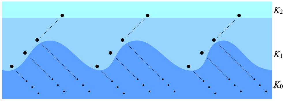
By definition, a subspace K of scattering height 3 that is scattered is such that K3 is empty, and also K is the (disjoint) union of K0, K1, and K2. Here is how such a space looks like. All the points of K2 are isolated inside K2, but are limits of nets of points from K1; this is what the sequences of dots (• • • ·······) on the K1 level mean. The points of K1 are themselves isolated in K1 ∪ K2 (= K’1), but are limits of nets of points from K0. All the involved nets are shown as completely separate here, but in general they can share points.
Proof. We will build a clopen selector for X. We reuse the notations K0, K1, K2, K’0, K’1, K’2 from above, with K≝X.
K2 only contains isolated points. For each x in K2, {x} is therefore open in K2. Since K2 = K’2 and K’2 is compact, we can extract a finite subcover from the cover of all singleton sets {x}, x in K2; it follows that K2 is in fact finite. (Oh, K’2 is compact… because I have said so above; if you had not realized that I had claimed so, read the post mentioned above on compact scattered subspaces!)
Let me list the points of K2 as x1, …, xn. We can find finitely many pairwise disjoint clopen subsets U1, …, Un (of K=X), such that each xi is in the corresponding Ui. This is why I spent all that time proving stuff about totally disconnected spaces! And that is simply Corollary G.
Then U1 ∪ … ∪ Un is clopen in X, so X–(U1 ∪ … ∪ Un) is also clopen in X: let me call that set U0. We have now found a partition of X in n+1 clopen sets U0, U1, …, Un. We define the desired clopen selector as follows:
- η(xi) ≝ Ui for every i, 1≤i≤n.
- For every point x in K1, there is a unique index i, 0≤i≤n, such that x ∈ Ui. Also, x is isolated in K’1 = K1 ∪ K2, so {x} is open in K’1, and this means that there is an open subset V of X such that V ∩ K’1 = {x}. Without loss of generality, namely by replacing V by V ∩ Ui if necessary, we may assume that V ⊆ Ui. By Proposition F, X has a base of compact-open subsets, so V contains a compact-open (hence clopen) neighborhood of x in X, and we define η(x) as that compact-open neighborhood.
We will need to note that, for every x ∈ K1,- (a) η(x) ⊆ Ui where i is the unique index i, 0≤i≤n, such that x ∈ Ui;
- (b) η(x) ∩ K’1 = {x}.
- For every point y of K0, y is isolated in X, so {y} is open in X; since X is Hausdorff hence T1, {y} is also closed, hence we are allowed to define η(y) as {y}.
Let us check the required properties.
- (DW0) for every point x of X, x ∈ η(x): obvious.
- (DW1) for all points x and y, x ∈ η(y) and y ∈ η(x) together imply x=y.
- If y is in K0, then η(y)={y}, so x ∈ η(y) already implies x=y; similarly, if x is in K0, then y ∈ η(x) implies x=y. Henceforth, let us assume that both x and y are outside K0.
- If y is in K2, then y=xi for some i with 1≤i≤n, and η(y)=Ui. There is no other point of K2 in Ui, so if x is in K2 and x ∈ η(y), then x=y. If x is in K1 then η(x) intersects K’1 = K1 ∪ K2 at x only by item (b) above, so y ∈ η(x) is impossible.
- Similarly if x is in K2, if x ∈ η(y) and y ∈ η(x) then x=y.
- Finally, if both x and y are in K1, then if x ∈ η(y), we obtain that x=y by item (b).
- (DW2) for all points x and y, if x ∈ η(y) then η(x) ⊆ η(y). Let us assume x ∈ η(y).
- If y is in K0, then η(y)={y}, and the only point of η(y) is y itself, so x=y, whence η(x) = η(y).
- If x is in K0, and then η(x)={x}, so η(x) = {x} ⊆ η(y). Henceforth, let us assume that both x and y are outside K0, that is, in K’1.
- If y is in K1, then by (b) the only point of η(y) that is also in K’1 is y, so x=y, whence η(x) = η(y).
- If y is in K2, then y=xi for some i with 1≤i≤n, and η(y)=Ui. Since x ∈ η(y), we have x ∈ Ui. If x is also in K2, then by definition of the sets Ui, y is the only point of K2 in Ui, so x=y, and therefore η(x) = η(y). If x is in K1 instead, then η(x) ⊆ Ui by item (a) above; and that means that η(x) ⊆ η(y). ☐
Acknowledgments
I wish to thank Christian Delhommé. He is the one who told me that what I was missing in Dow and Watson’s proof of their Corollary 1 (in [2]) was the fact that every scattered T1 space is totally disconnected, hence had a base of clopen subsets.
- Hoffmann, Rudolf-Eberhard. On the Sobrification Remainder sX–X. Pacific Journal of Mathematics, 83(1):145–156, 1979.
- Alan Dow and Stephen Watson. Skula spaces. Commentationes Mathematicae Universitatis Carolinae 31(1):27–31, 1990. ISSN: 0010-2628.
- Jean Goubault-Larrecq and Maurice Pouzet. A few characterizations of topological spaces with no infinite discrete subspace. Topology and its Applications 341, January 1st 2024, 108733.

— Jean Goubault-Larrecq (January 21st, 2024)