
Great news this month! Yuxu Chen, Hui Kou and Zhenchao Lyu, from the University of Sichuan in Chengdu, have finally cracked the problem whether FS-domains and RB-domains are the same notion [1], and they are not. This problem had been open since the invention of FS-domains by Achim Jung in 1990 [2]. Every RB-domain is an FS-domain, and the issue was the reverse inclusion. In the same paper [2], Achim Jung mentions a possible counterexample to the reverse inclusion, suggested by Jimmie Lawson: the FS-domain Disc of discs in the plane. I have covered this in the April 2018 post. And this is exactly what Chen, Kou and Lyu show: Disc is not an RB-domain.
The challenge was tough. There is no easy way to prove that a given dcpo is not an RB-domain, other than showing that it does not obey one of the properties that all RB-domains satisfy. For example, all RB-domains are stably compact in their Scott topology. But all FS-domains are, too, so it is hopeless to try and show that Disc is not an RB-domain by attempting to show that it is not stably compact: it simply is.
Accordingly, the proof by Chen, Kou and Lyu is very inventive, and goes through a series of mathematical tools not usually considered in domain theory. These mathematical tools are nonetheless well-known.
- There is Carathéodory’s theorem in convex geometry of finite dimensional real vector spaces Rn: every point that is in the convex hull of a set S in Rn, namely that is a finite convex combination ∑i=1m ai . xi where each xi is in S, each ai is non-negative and ∑i=1m ai=1, is already a finite convex combination of at most n+1 points of S.
- There is quite a lot of basic 3 × 3 matrix algebra.
- There is a lot of university level topology, inside spaces of the form Rn or included in such a space, where, rather comfortably, you can reason with convergence of sequences (not nets) and limits are unique.
- There is a lot of basic measure theory: Lebesgue measurable sets, Lebesgue’s dominated convergence theorem, the Tonelli-Fubini theorem.
- And finally, there is Rademacher’s theorem: For every open subset U of Rn and for every Lipschitz continuous map f : U → Rm, f is differentiable almost everywhere in U; that is, the points in U at which f is not differentiable form a set N of Lebesgue measure zero. Then the gradient ∇f is defined at every point of U outside of N. Letting f map every x ∈ U to (fi (x))1≤i≤m, ∇f is the map from U to the set Mat(m, n) (= Rm × n) of m × n matrices defined by ∇f(x) ≝ (∂fi (x)/∂xj)1≤i≤m, 1≤j≤n. The existence of ∇f is stronger than the mere existence of the partial derivatives ∂fi (x)/∂xj: it says that f(y) = f(x) + ∇f(x).(y–x) + o (|y–x|) as y tends to x in U, including when y is not required to follow an xj-axis.
For Rademacher’s theorem, Chen, Kou and Lyu cite Theorem 3.2] of [3]. The proof there, which is due to Charles Morrey if I am not wrong, makes it clear that if f is 1-Lipschitz, then the directional derivative ∇f(x).v along any vector v of norm 1 has norm at most 1. We will use the Euclidean (or L2) norm on Rm and on Rn, and the Euclidean norm of a vector v will be written as |v|. The previous sentence shows that for a 1-Lipschitz map f on U, the linear operator ∇f(x)—at each point x where it is defined—has sup norm ||∇f(x)|| ≤ 1: the sup norm is the supremum of |∇f(x).v| over all vectors v of norm 1, by definition.
While this can seem impressive, the real novelty is the idea of going from something that Chen, Kou and Lyu call the matrix cone RC of a certain well-known cone, the Lorentz cone C. Showing that a certain matrix-valued integral lies in RC is also technically difficult. I will make my best to explain all that below. I will make a few simplifications along the way, but the general structure of the proof will remain what Chen, Kou and Lyu have set out.
Disc, formal balls, and the Lorentz cone
The object of study here is Disc: the poset of all closed discs in R2, plus R2 itself, ordered by reverse inclusion (so R2 is the bottom element of Disc). We have seen in the April 2018 post that Disc is an FS-domain, in fact that it is isomorphic to B(R2, d)⊥, where B(R2, d) is the poset of formal balls of R2 with distance d(x,y) ≝ |y–x|; the ⊥ subscript means that we have added a bottom element ⊥ below all formal balls. A formal ball is simply a pair (x, r) where x is a point of R2 and r (the radius) is a non-negative real number. They are ordered by (x, r) ≤d (y, s) if and only if d(x,y) ≤ r–s.
We can equate B(R2, d) with the product H ≝ ]–∞, 0] × R2, by mapping a formal ball (x, r) to the pair (–r, x). Then (x, r) ≤d (y, s) if and only if the difference (–s, y) – (–r, x) is in a very classical mathematical object, the Lorentz cone C ≝ {(t, z) ∈ R × R2 | t ≥ |z|}. This is the region of 3-dimensional space above the surface shown below:
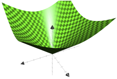
This is the Lorentz cone in 3 dimensions. It is easier to understand what it looks like in 2 dimensions, and this is the gray region depicted below.
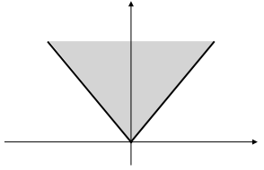
I will include a few pictures below, and they will be 2-dimensional, because that makes it easier to understand them. Most of the mathematics works in any dimension. But beware that the dimension 2 case can be deceivingly simple. It would arise from the consideration of discs on the line R rather than on the plane R2, and discs on the line are just closed intervals; but the domain of closed intervals ordered by reverse inclusion is an RB-domain, even a bc-domain. Hence something more subtle happens on the plane, or equivalently with the Lorentz cone in dimension 3 or higher.
The Lorentz cone is a cone, and we need to say what that means. A cone is a subset of a real vector space that is closed under convex combinations and multiplication by non-negative scalars (hence under all linear combinations with non-negative coefficients). Some people call such a thing a convex cone.
Every cone defines a preordering ≤C on a containing vector space (or any subset, such as H) by z ≤C z’ if and only if z’–z is in C. This is a partial ordering if there is no vector z that is in C such that –z is in C, too, except for the zero vector.
Up to the isomorphism between B(R2, d) and H, we are interested in the poset H ordered by the cone ordering ≤C, where C is the Lorentz cone. Since B(R2, d) is a dcpo when ordered by ≤d (this comes from the fact that R2 is a complete metric space under d), H is a dcpo when ordered by ≤C. What Chen, Kou and Lyu show is that H⊥ (H with an extra bottom element ⊥) is not an RB-domain.
In the rest of this post, we will assume that H⊥ is an RB-domain, and we will obtain a contradiction, replaying Chen, Kou and Lyu’s argument. Their paper [1] is remarkably detailed and relatively easy to follow. I will occasionally simplify some of their arguments—in general at the price of generality—but the changes I will make are small.
Since H⊥ is an RB-domain, by definition, there is a directed family (ri)i ∈ I of deflations on H⊥ whose (pointwise) supremum is the identity map. That ri is a deflation means that ri is Scott-continuous, and has finite image.
I have said that we would order H = ]–∞, 0] × R2 with the cone ordering, but I have not said which topology we would consider on it. We will not consider the Scott topology, rather the usual metric topology. With this topology, the interior int(H) is ]–∞, 0[ × R2.
Similarly, we will give C its usual metric topology. The interior int(C) of C is {(t, z) ∈ R × R2 | t > |z|}. This is an important set because of the following.
Fact A. In H, x ≪ y (x is way-below y) if and only if y–x is in int(C).
Proof. Equivalently, this means that given two formal balls (x, r) and (y, s) on R2, (x, r) ≪ (y, s) if and only if d(x,y) < r–s. This property holds on the space of formal balls of any Smyth-complete quasi-metric space, by the Romaguera-Valero theorem (Theorem 7.3.11 in the book), and every complete metric space, for example R2, is certainly a Smyth-complete quasi-metric space (see Lemma 7.2.5 in the book). ☐
We will now consider a fixed but arbitrary compact rectangle P in int(H) with non-empty interior, namely a product [–b, –a] × [c, d] × [e, f], with –∞<–b<–a<0, and c<d and e<f in R. Every compact rectangle is compact in H, with its usual metric topology.
The following is Lemma 3.1 in [1]. Instead of calling it Lemma A (or Lemma B), as I usually do, I will simply keep the numbering of the paper. We note that the vector e ≝ (1, 0, 0) is in int(C).
Lemma 3.1 [1]. (Under the assumption that Disc is an RB-domain.) Let P be a compact rectangle in int(H) with non-empty interior. For every ε>0, there is a map Qε : P → H such that:
- Qε is monotonic in the cone ordering ≤C;
- Qε has finite image;
- for every vector x in P, Qε(x) is in the closed interval [x–ε.e, x], namely: x–ε.e ≤C Qε (x) ≤C x.
In particular, Qε(x) converges uniformly to x on P as ε tends to 0.
Proof. As one would rightly guess, Qε will be ri for a suitable index i ∈ I. One difficulty is that ri may take the value ⊥, but Qε is not allowed to, since its values have to be in H.
Since ri is Scott-continuous, it is in particular monotonic—with respect to ≤C—so property 1 will be automatic. Property 2 will be, too. We only have to find i so that property 3 holds. For every x ∈ P, x–3ε/4.e ≪ x–ε/2.e by Fact A, remembering that e ≝ (1, 0, 0) is in int (C). Since x–ε/2.e is the supremum of the directed family ri (x–ε/2.e), i ∈ I, in H⊥, there is an index ix in I such that x–3ε/4.e ≤C rix (x–ε/2.e). The set Nx of all points y in H such that x–y+ε/4.e and y–x+ε/2.e are in int(C) is open in H, since int(C) is open and addition and multiplication are continuous.
Then Nx is an open neighborhood of x, since ε/4.e and ε/2.e are in int(C). Since P is compact, finitely many Nx cover P. In other words, there is a finite set E of points of P such that P ⊆ ∪x ∈ E Nx. Let i ∈ I be such that rix ≤ ri for every x ∈ E. This is the desired i.
Then x–3ε/4.e ≤C ri (x–ε/2.e) for every x ∈ E. We check that for every y ∈ P, y–ε.e ≤C ri (y) ≤C y. In particular, this will entail that ri (x) ≠ ⊥, so defining Qε as ri gets us a function with values in H, not H⊥. Let us verify the two desired inequalities. Since y ∈ P, there is a point x ∈ E such that y ∈ Nx. By definition of Nx and since int(C) ⊆ C, we obtain : (1) x–y+ε/4.e ∈ C and (2) y–x+ε/2.e ∈ C.
- We have x–y+ε/4.e = (x–3ε/4.e) – (y–ε.e), which is in C by (1); so y–ε.e ≤C x–3ε/4.e. We remember that x–3ε/4.e ≤C ri (x–ε/2.e).
- By (2), x–ε/2.e ≤C y. Since ri is monotonic, it follows that ri (x–ε/2.e) ≤C ri (y). Combining this with the previous point, y–ε.e ≤C ri (y).
- We have ri (y) ≤C y because ri is below the identity. ☐
Let me add the following piece of information. Chen, Kou and Lyu show that every function that is monotonic with respect to the cone ordering ≤C and has finite image is Lebesgue measurable [1, Proposition 5.3], but we can say this and a bit more about Qε without a lot of effort. Let me write ↑C for upward closure in the cone ordering.
Lemma B. For every ε>0, for every y in the image Im Qε of Qε, Qε–1(↑C y) is open in H (with its usual metric topology) and upwards-closed with the cone ordering ≤C. Qε–1({y}) is the difference of two upwards-closed open subsets of H.
Proof. Qε–1(↑C y) is upwards-closed because Qε is monotonic.
We recall that Qε is equal to ri for some i ∈ I, suitably restricted to P. There is a Scott-open subset U of H⊥ whose intersection with Im Qε is ↑C y: we simply take the complement of the downward closure of the finite set Im Qε – ↑C y. Then ri–1(↑C y) is Scott-open in H⊥, since ri is Scott-continuous. We can therefore write it as a union of sets ↟x, where x ranges over ri–1(↑C y) (see Theorem 5.1.17 in the book), since H⊥ is isomorphic to the continuous dcpo B(R2, d)⊥, and is itself a continuous dcpo. None of the points x can be equal to ⊥, otherwise ⊥ = ri(⊥) would be in ↑C y, which is impossible, since y is in Im Qε ⊆ H.
By Fact A, ↟x is equal to {z ∈ H | z–x ∈ int(C)}. Since int(C) is obviously open (by definition of interiors) in H and subtraction is continuous, ↟x is open in H. Any union of open sets is open, so ri–1(↑C y) is open in H—with the metric topology, let us stress it.
Now Qε–1(↑C y) = ri–1(↑C y) ⋂ P, so Qε–1(↑C y) is open in P. For the final claim, we note that Qε–1({y}) = Qε–1(↑C y) – ∪z Qε–1(↑C z), where the latter union is over the finitely many elements z of Im Qε that are strictly larger than y in the cone ordering. ☐
Now our task reduces to showing that such monotonic maps Qε with finite image cannot exist. We can safely forget about RB-domains and formal balls. We will only reason on H, C and derived constructions. Here is the main such derived construction.
3 × 3 matrices, and the matrix cone RC
Let Mat(m, n) be the set of m × n matrices. This is an mn-dimensional real vector space. We will focus on Mat(3, 3), a 9-dimensional vector space. We give it the usual metric topology of R9.
We see every vector v in R3 as a column vector, with its first element v1 on top, its second element v2 in the middle, and its third element v3 at the bottom. Hence v = (v1 v2 v3)T where the T superscript means “transpose”. This also means that e ≝ (1, 0, 0) is really (1 0 0)T.
For every pair of vectors v, w in R3, we can form a 3 × 3 matrix v wT: its entries are just viwj, where 1≤i, j≤3. Explicitly, writing v as (v1 v2 v3)T and w as (w1 w2 w3)T (the T superscript is meant to remind you that v and w should be column vectors, not row vectors), v wT is the matrix .
Such matrices are very special, and I will call them generators. They have rank 1 (or 0, for the all-zero matrix). We let RC be the smallest cone that contains every matrix v wT with v, w in the Lorentz cone C. Its elements are the finite linear combinations ∑i=1m ai . vi wiT, where m ∈ N, each ai is a positive real number, and each vi and each wi is an element of C. RC is the matrix cone associated with C.
RC is a standard construction. Every matrix of rank 1 is of the form v wT for two vectors v, w (not necessarily in C), and then the singular value decomposition procedure shows that every square matrix is a finite linear combination of such matrices. The difference here is that, in building the linear combinations ∑i=1m ai . vi wiT in RC, we also require that each vi and each wi is in C.
All this has the following interpretation in Einstein’s special relativity. If you interpret the first component v1 of a vector (v1 v2 v3)T as time and the other two as space coordinates, C is the cone of vectors that you can reach from the zero vector by traveling at a speed that does not exceed 1 (the “speed of light”, after renormalizing it to 1) in norm. C is sometimes called the future causal cone, and the ordering ≤C is the causal ordering: considering that you cannot exceed the speed of light, any two states v and w of the same particle must be such that v ≤C w or w ≤C v; v occurs before w in the first case, and otherwise w occurs before v. Then RC is a class of linear transformations that preserve causality, because they all map vectors of C to C.
Proposition 4.1 [1]. The cone RC is closed in Mat(3, 3).
Proof. Let us say that v = (t, z) ∈ C (with t ∈ R, z ∈ R2, and t ≥ |z|) is normalized if and only if t=1. A generator is normalized if one can write it as v wT where both v and w are normalized. Let me call an element of RC normalized if and only if one can write it as ∑i=1m ai . vi wiT where each vi and each wi is normalized and ∑i=1m ai = 1. Namely, such matrices are convex combinations of normalized generators. Let me write RC1 for the collection of normalized elements of RC.
By definition, RC1 is convex. Hence, by Carathéodory’s theorem, every element of RC1 is the convex combination of at most 10 normalized generators. We can require the number of generators to be exactly 10, by adding dummy terms with ai=0. The set of normalized elements of C is closed and bounded in R3, hence it is compact. Similar, the set of row vectors (a1 … a10) of non-negative real numbers summing up to 1 (the 9-dimensional simplex) is compact. The function that maps any such row vector and any 10-tuple of pairs of normalized elements vi and wi of C to ∑i=110 ai . vi wiT is continuous, so RC1 is compact.
Now RC is exactly the collection of matrices of the form λ M where λ ∈ R+ (the set of non-negative reals) and M ∈ RC1. Let us call that the standard form of an element of RC. This is easy to obtain: the component in row 1 and colum 1 of any element of RC1 is equal to 1, so we can read off λ from the (1, 1) entry of any given matrix ∑i=1m ai . vi wiT in RC. We assume that every ai is non-zero. Let ti be the first component of vi, so that vi = ti v’i where v’i is normalized; similarly, let si be the first component of wi, so that wi = si w’i where w’i is normalized. If λ=0, then every ti and every si is equal to 0, so every vi and every wi is the zero vector by definition of C, our matrix is the zero matrix, and can therefore be written as λ M where, say, M = (1 0 0) (1 0 0)T (or any other element of RC1). Otherwise, ∑i=1m ai . vi wiT = λ ∑i=1m aitisi/λ . v’i w’iT. It remains to verify that ∑i=1m aitisi/λ = 1, equivalently that ∑i=1m aitisi = λ: this is clear, because both sides are equal to the (1, 1) entry of ∑i=1m ai . vi wiT.
In order to see that RC is closed, we consider any sequence (λn Mn)n ∈ N of elements of RC in standard form and we assume that it converges to some matrix λ M of Mat(3, 3). (We take λ to be the (1, 1) entry of the limit matrix, so that the (1, 1) entry of M is 1.) We wish to show that λ M is in RC. If λ=0, this is clear, since the zero matrix is in RC. Let us therefore assume that λ≠0. Since (λn Mn)n ∈ N converges to λ M, in particular the (1, 1) entries of the matrices λn Mn, which are simply the numbers λn, converge to the (1, 1) entry λ of λ M. Therefore 1/λn converges to 1/λ as n tends to infinity, and since product is jointly continuous, 1/λn (λn Mn) converges to 1/λ (λ M) as n tends to infinity. In other words, Mn tends to M as n tends to infity. But every Mn is in RC1, RC1 is compact, hence closed because Mat(3, 3) is Hausdorff, and therefore M is in RC1. Therefore λ M is in RC. We have shown that RC is closed under taking limits of arbitrary convergent sequences, namely it is sequentially closed. Hence RC is closed. (The fact that sequentially closed sets are closed holds more generally in any first-countable space, see Exercise 4.7.14 in the book). ☐
The last paragraph of the proof above replaces a more complicated argument in [1], but the overall structure of the proof is the same. I should say that the fact that RC is closed seems to be well-known, as an Internet search tells me. Notably, the classic textbook by Ralph Tyrell Rockafellar, Convex Analysis, Princeton University Press, 1970 (https://doi.org/10.1515/9781400873173) apparently has it—but I don’t have that book, and therefore I cannot confirm.
Test functions
For every C1 function ψ : Ω → R, where Ω is an open subset of Rn, its gradient ∇ψ : Ω → Rn is defined as mapping every x ≝ (x1 … xn) ∈ Ω to the vector ∇ψ(x) ≝ (∂ψ (x)/∂xj)1≤j≤n of the partial derivatives of ψ at x. (C1 means that the partial derivatives exist and are continuous in x.)
Concretely, we will need just one such function ψ on R3. We may require ψ to be C∞, as Chen, Kou and Lyu do, but this is not necessary. Here is the concrete construction we shall use.
- Given any real interval [α, β] with α<β, let B’[α, β] be defined as mapping every x outside [α, β] to 0 and every x ∈ [α, β] to –2π/(β–α)2 sin (2π (x–α)/(β–α) — π). The funny constant –2π/(β–α)2 is rettrofitted to make everything below work.
- We integrate B’[α, β], and we find that B’[α, β] is the derivative of a function B[α, β] that maps every x outside [α, β] to 0 and every x ∈ [α, β] to 1/(β–α) + 1/(β–α) cos (2π (x–α)/(β–α) — π). B[α, β] is C1, and takes non-negative values. I will call this the bump function, and I have displayed it in the picture below. (There are a lot of alternative ways to define a similar bump functions. We are just happy to have one here.)
- Integrating B[α, β] on [α, β], or equivalently on the whole of R, or any interval I that contains [α, β], we obtain that the integral is equal to [1/(β–α) x + 1/2π sin (2π (x–α)/(β–α) — π)]αβ, where the […]αβ notation means the value of the function between square brackets taken at β minus its value taken at α. The sine terms vanish, and we are left with 1. In other words, ∫I B[α, β] dx = 1.
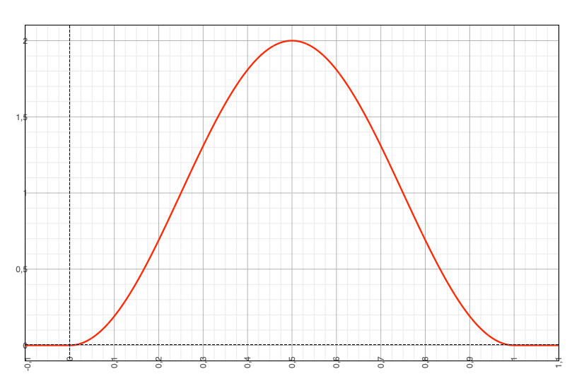
Whatever α<β, B[α, β] is C1, non-negative valued, vanishes outside [α, β], and has integral equal to 1.
We recall that the functions Qε of Lemma 3.1 [1] (see above) are defined on a compact rectangle P = [–b, –a] × [c, d] × [e, f]. We define ψ(x) as B[–b, –a] (x1) B[c, d] (x2) B[e, f] (x3) for every x = (x1 x2 x3) ∈ P. We note that ∫P ψ(x) dx = ∫–b–a B[–b, –a] (x1) dx1 ∫cd B[c, d] (x2) dx2 ∫ef B[e, f] (x3) dx3 = 1.
In passing, I used to write elements of P as (t, z) ∈ R × R2, and I have started to write them as (x1 x2 x3). I will use one or the other notation; you will have to remember that t=x1 and that z=(x2 x3).
We now form the integral ∫P Qε(x) ∇ψ(x)T dx. This is the integral of a function with values in Mat(3, 3) = R9, which we take as shorthand for the matrix of the integrals of the 9 corresponding functions. Well, we will have to add a minus sign, really, and therefore we consider the opposite –∫P Qε(x) ∇ψ(x)T dx.
The idea of the remainder of the proof is to show that:
- –∫P Qε(x) ∇ψ(x)T dx is in the matrix cone RC for every ε>0;
- –∫P Qε(x) ∇ψ(x)T dx tends to the 3 × 3 identity matrix I3, hence I3 is in RC, since RC is closed by Proposition 4.1 [1] (which we reproved above);
- but I3 is in fact not in RC.
I have designed this post so that you can stop here and get a good idea how Chen, Kou and Lyu proceed. If you are brave, the next section is about proving point 1 above. This is definitely the difficult part, and the part where Rademacher’s theorem is used. Points 2 and 3 are easy, and you can scroll all the way to the bottom of this post in order to see how this is proved.
–∫P Qε(x) ∇ψ(x)T dx is in the matrix cone RC
Since the image Im Qε of Qε : P → H is finite, we can write Qε as the finite sum ∑y ∈ Im Qε y . χEy, where Ey is the inverse image of y under Qε, namely Ey ≝ Qε–1 ({y}). We see each y as a column vector, as usual. The notation y . χEy denotes the map that sends every element of Ey to y and every element outside of Ey to the zero vector.
Then –∫P Qε(x) ∇ψ(x)T dx = –∑y ∈ Im Qε y (∫P χEy (x) ∇ψ(x) dx)T is in RC, by definition of RC. This looks like what we need: a finite sum ∑i=1m ai . vi wiT, but we are far from the goal. First, there is this nasty minus sign in front of the sum. More importantly, the terms y and ∫P χEy (x) ∇ψ(x) dx used in the sum are not in C. Oops. Hence we will rearrange the sum.
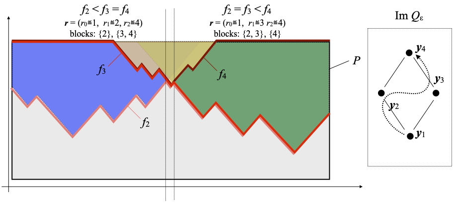
Let us have a look at what Qε looks like. Below, I have drawn a typical situation, where Im Qε has four elements. I have made sure that the elements of Im Qε are partially, not totally ordered, and this is depicted on the right part of the picture. (This will indeed be a difficulty.) I have drawn the rectangle P on the left, in 2 dimensions instead of 3 for readability. The four colored regions are the inverse images Qε–1(↑C y), suitably intersected with P, when y ranges over the four points of Im Qε.
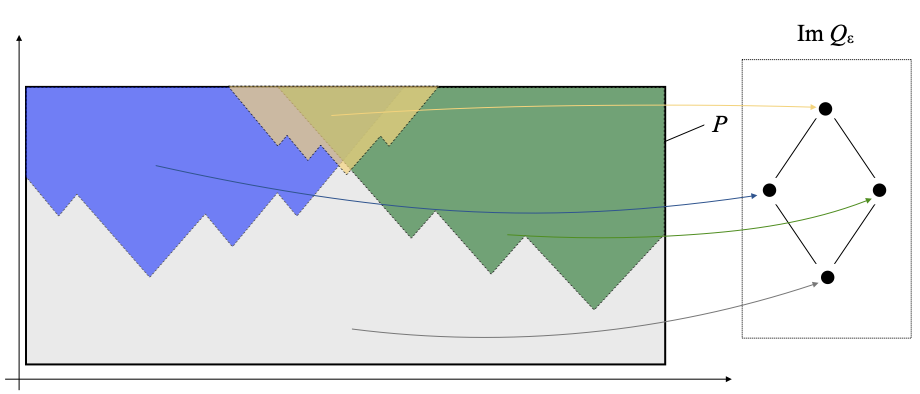
The regions Qε–1(↑C y) are upwards-closed and open by Lemma B. I have shown their lower boundaries as jagged curves, because there is no reason that they should be the graphs of differentiable functions. But they are graphs of 1-Lipschitz functions, as Chen, Kou and Lyu observe: in other words, the slope of these curves cannot exceed 1 in absolute value.
The following is Lemma 5.1 of [1], more or less. Let me recall that P = [–b, –a] × [c, d] × [e, f].
Lemma C. For every subset U of P that is upwards-closed in ≤C, there is a unique 1-Lipschitz map f : [c, d] × [e, f] → [–b, –a] such that every point x ≝ (x1 x2 x3)T,
- if x ∈ U, then f (x2, x3) ≤ x1;
- if f (x2, x3) < x1 then x ∈ U.
In other words, U is exactly the set of points x such that f (x2, x3) ? x1, where ? means ≤ or <. We will then write U as Uf to make the 1-Lipschitz map f explicit in the sequel, although there are in general more than one open set U associated with the same map f. But this will not be important.
Proof. Let U be upwards-closed in C. For every pair (x2, x3) in [c, d] × [e, f], if f exists as indicated, then f (x2, x3) has to be the infimum of all the values x1 ∈ [–b, –a] such that (x1 x2 x3)T is in U, where we agree that the infimum of an empty set of values in [–b, –a] is –a. This shows that f is unique if it exists. In order to show existence, we define f (x2, x3) as the infimum of all the values x1 ∈ [–b, –a] such that (x1 x2 x3)T is in U for every pair (x2, x3) in [c, d] × [e, f].
- If (x1 x2 x3)T ∈ U, then by definition of f, x1 ≥ f (x2, x3).
- If f (x2, x3) < x1, then by definition of f there is a number t ∈ [–b, –a] such that (t x2 x3)T ∈ U and t < x1. But then (x1 x2 x3)T = (t x2 x3)T + (x1–t).e, where you may recall that we have defined e ≝ (1 0 0)T, and e is in int(C), in particular in C. Therefore (x1 x2 x3)T ≥C (t x2 x3)T. Since U is upwards-closed in ≤C, (x1 x2 x3)T is in U.
(Oops, I forgot this in the first version of this post; added the same day, July 14th, 2026:) Finally, we must show that f is 1-Lipschitz, namely that |f (x2, x3) – f (y2, y3)| ≤ |(x2, x3) – (y2, y3)| for all (x2, x3) and (y2, y3) in [c, d] × [e, f]. Without loss of generality, we assume that f (x2, x3) ≤ f (y2, y3). We have to show that f (y2, y3) – f (x2, x3) ≤ |(x2, x3) – (y2, y3)|. For every ε>0, the vector (f (x2, x3)+ε x2 x3)T is in U by the second item proved in this lemma. By definition of ≤C, we have (f (x2, x3)+ε x2 x3)T ≤C (f (x2, x3)+ε+|(x2, x3) – (y2, y3)| y2 y3)T. Now U is upwards-closed, so (f (x2, x3)+ε+|(x2, x3) – (y2, y3)| y2 y3)T is also in U. By the first item of this lemma, f (y2, y3) ≤ f (x2, x3)+ε+|(x2, x3) – (y2, y3)|. Since ε>0 is arbitrary, f (y2, y3) ≤ f (x2, x3)+|(x2, x3) – (y2, y3)|, which is what we wanted to prove. ☐
We now evaluate ∫P χU (x) ∇ψ(x) dx for an arbitrary upwards-closed subset U of P. This is essentially Lemma 5.2 of [1]. Chen, Kou and Lyu do this in a more general setting than we do: we are only using a very simple test function ψ, defined by ψ(x) ≝ B[–b, –a] (x1) B[c, d] (x2) B[e, f] (x3), and this will allow us to use elementary facts about integration on the real line instead of the Gauss-Green formula. The fact that ∇f (z) exists for almost every z, hence also that ∂f (x2, x3)/∂x2 and ∂f (x2, x3)/∂x3 exist for almost every z–namely for every z except on a set of Lebesgue measure 0–is by Rademacher’s theorem. Technically, Rademacher’s theorem applies for functions defined on an open set, not on a compact rectangle such as P, but the functions we integrate below extend to the whole of R3, and are 0 outside of P. It is well-known that Lebesgue integrals are impervious to changes in the integrated function made on a set of Lebesgue measure 0.
Lemma D. For every upwards-closed subset of P, which we write as Uf as given in Lemma C, for a unique 1-Lipschitz map f,
–∫P χUf (x) ∇ψ(x) dx = ∫[c, d] × [e, f] ψ (f (z), z) (1, –∇f (z))T dz
where z is shorthand for a pair (x2, x3). In other words, the right-hand side is equal to:
∫[c, d] × [e, f] ψ ((f (x2, x3) x2 x3)T) (1 –∂f (x2, x3)/∂x2 –∂f (x2, x3)/∂x3)T dx2 dx3
Proof. We check each coordinate.
- Coordinate 1 of –∫P χUf (x) ∇ψ(x) dx is –∫P χUf (x) ∂ψ(x)/∂x1 dx = –∫cd B[c, d] (x2) ∫ef B[e, f] (x3) ∫f (x2, x3)–a B’[–b, –a] (x1) dx1 dx3 dx2 (using the Tonelli-Fubini theorem). Note the lower bound of integration on x1 set to f (x2, x3): the term ∫f (x2, x3)–a B’[–b, –a] (x1) dx1 is obtained by simplifying the actual term the definition gets us, which is ∫–b–a χI B’[–b, –a] (x1) dx1, where I is the interval of all x1 ∈ [–b, –a] such that f (x2, x3) ? x1, where ? is ≤ or <; and whether I is the half-open interval ]f (x2, x3), –a] or the whole interval [f (x2, x3), –a], ∫–b–a χI B’[–b, –a] (x1) dx1 = ∫f (x2, x3)–a B’[–b, –a] (x1) dx1.
Now we compute ∫f (x2, x3)–a B’[–b, –a] (x1) dx1 = B[–b, –a] (–a) – B[–b, –a] (f (x2, x3)) = –B[–b, –a] (f (x2, x3)), since B[–b, –a] (–a) = 0.
Therefore the first coordinate of –∫P χUf (x) ∇ψ(x) dx is ∫cd B[c, d] (x2) ∫ef B[e, f] (x3) B[–b, –a] (f (x2, x3)) dx1 dx2 dx3 = ∫[c, d] × [e, f] ψ ((f (x2, x3) x2 x3)T) dx2 dx3. - Coordinate 2 of –∫P χUf (x) ∇ψ(x) dx is –∫P χUf (x) ∂ψ(x)/∂x2 dx = –∫ef B[e, f] (x3) ∫cd B’[c, d] (x2) ∫f (x2, x3)–a B[–b, –a] (x1) dx1 dx2 dx3 (using Tonelli-Fubini, this time with a different order of integration). For every x3, the inner double integral ∫cd B’[c, d] (x2) ∫f (x2, x3)–a B[–b, –a] (x1) dx1 dx2 is the simple integral ∫cd B’[c, d] (x2) F (f (x2, x3)) dx2 where F (t) ≝ ∫t–a B[–b, –a] (x1) dx1. By the fundamental theorem of calculus, F is differentiable, and F’ (t) = –B[–b, –a] (t) for every t ∈ R. We integrate by parts: ∫cd B’[c, d] (x2) F (f (x2, x3)) dx2 = [B[c, d] (x2) F (f (x2, x3))]cd – ∫cd B[c, d] (x2) F’ (f (x2, x3)) ∂f (x2, x3)/∂x2 dx2.
The term [B[c, d] (x2) F (f (x2, x3))]cd is equal to 0 because B[c, d] (c) = B[c, d] (d) = 0. The remaining term is equal to ∫cd B[c, d] (x2) B[–b, –a] (f (x2, x3)) ∂f (x2, x3)/∂x2 dx2.
Putting back the outer integral –∫ef B[e, f] (x3) … dx3, it follows that the second coordinate of –∫P χUf (x) ∇ψ(x) dx is equal to –∫ef B[e, f] (x3) ∫cd B[c, d] (x2) B[–b, –a] (f (x2, x3)) ∂f (x2, x3)/∂x2 dx2 dx3, and this is equal to ∫[c, d] × [e, f] ψ ((f (x2, x3) x2 x3)T) × (–∂f (x2, x3)/∂x2) dx2 dx3. - Similarly, the third coordinate of –∫P χUf (x) ∇ψ(x) dx is equal to ∫[c, d] × [e, f] ψ ((f (x2, x3) x2 x3)T) × (–∂f (x2, x3)/∂x3) dx2 dx3. ☐
Things are starting to look good: we are starting to see some elements of C appear, as the following lemma shows.
Lemma D. For almost every z ≝ (x2, x3) (namely, for every z except on a set of Lebesgue measure 0), the vector (1, –∇f (z)) = (1 –∂f (x2, x3)/∂x2 –∂f (x2, x3)/∂x3) is in C.
Proof. When I recalled Rademacher’s theorem at the beginning of this post, I said that ||∇f(z)|| ≤ 1 whenever ∇f(z) is defined, which happens for almost every z. The sup norm ||∇f(z)|| is the supremum of |∇f(x).v| over all vectors v of Euclidean norm 1, by definition. We claim that ||∇f(z)|| is equal to the Euclidean norm |∇f(z)|. More generally, for every 2-dimensional vector (a, b), we claim that ||(a, b)|| = |(a, b)|. For every vector v such that |v|=1, |(a, b) . v| ≤ |(a, b)| . |v| by the Cauchy-Schwarz inequality, so taking suprema and recalling that |v|=1, ||(a, b)|| ≤ |(a, b)|. Another aspect of the Cauchy-Schwarz inequality is that the supremum over all v is attained when v and (a, b) are collinear. In other words, let v ≝ (a/|(a, b)|, b/|(a, b)|). Then |(a, b) . v| = |(a, b)|, showing that |(a, b)| ≤ ||(a, b)||. This argument fails if a=b=0, in which case ||(a, b)|| = |(a, b)| is obvious anyway.
Hence we really have that |∇f(z)| ≤ 1 whenever ∇f(z) is defined, and this is exactly what we need to state that (1, –∇f (z)) is in C. ☐
We now look at Qε. Let us fix a topological sort y1, …, yN of the elements of Im Qε, namely an enumeration of the elements of Im Qε such that for all indices i, j ∈ {1, …, N}, if yi ≤ yj then yi occurs before yj in the list, that is, i ≤ j. Here is a picture of one possible topological sort of our previous example. The other one would list y2 and y3 the other way around.
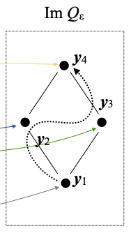
I will let you convince yourself that such a topological sort always exists. In fact, every partial ordering (on any set, even an infinite set) can be extended to a total ordering: this is the Szpilrajn extension theorem. (Chen, Kou and Lyu do something in the same spirit, but more ad hoc, at the beginning of their proof of Proposition 5.3 [1].)
Lemma E. We can write Qε as y1 + ∑k=2N (yk – yk–1) . χUfk, where f2 ≤ … ≤ fN is a monotone sequence of 1-Lipschitz maps from [c, d] × [e, f] to [–b, –a].
The proof is below. Before we come to it, in the example we have used until now, there are three 1-Lipschitz maps f2 ≤ f3 ≤ f4, and they are as shown below.
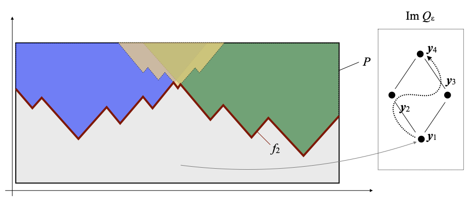
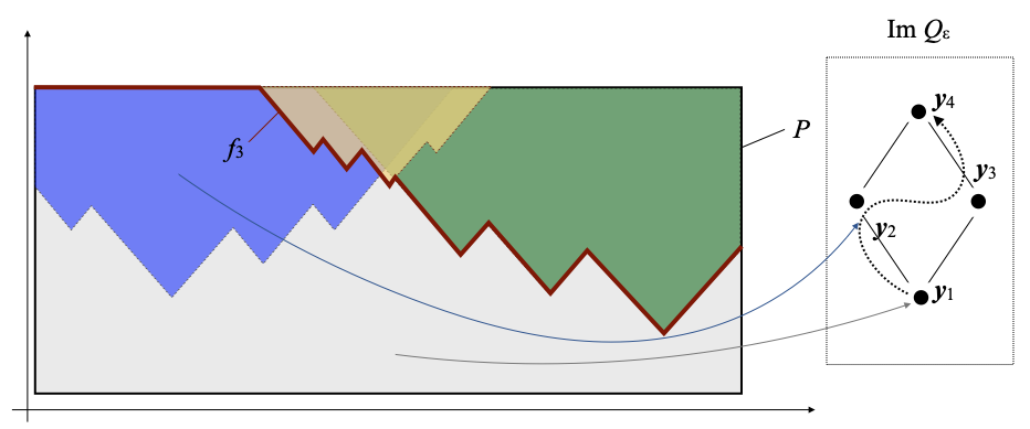
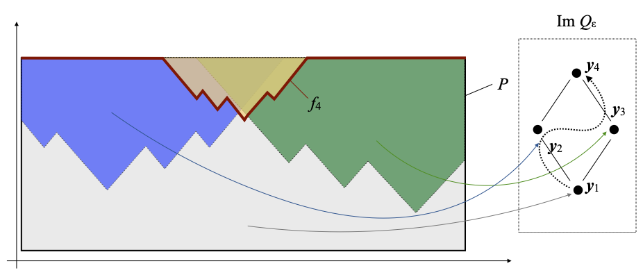
Proof. For every k ∈ {2, …, N}, by Lemma B Qε–1(↑C yk) ∪ … ∪ Qε–1(↑C yN) is open and upwards-closed, hence of the form Ufk for some unique 1-Lipschitz map fk from [c, d] × [e, f] to [–b, –a]. As k increases, the sets Qε–1(↑C yk) ∪ … ∪ Qε–1(↑C yN) get smaller and smaller, so f2 ≤ … ≤ fN. It remains to show that Qε (x) = y1 + ∑k=2N (yk – yk–1) . χUfk (x) for every x ∈ P. By definition, Qε (x) is equal to yp for some p ∈ {1, …, N}. Then:
- x is in Qε–1(↑C yk) ∪ … ∪ Qε–1(↑C yN) for every k ∈ {1, …, p}, simply because the union contains the term Qε–1(↑C yp).
- Also, x is not in Qε–1(↑C yk) ∪ … ∪ Qε–1(↑C yN) for any k ∈ {p+1, …, N}: otherwise x would be in Qε–1(↑C yk’) for some k’ ≥ k > p, so yp = Qε (x) would be larger than or equal to yk’, where k’ > p; this is impossible, since by definition of topological sorts, yp ≥ yk’ implies p ≥ k’.
Hence, in the sum ∑k=2N (yk – yk–1) . χUfk (x), χUfk (x) is equal to 1 for k varying between 2 and p, and to 0 for the remaining values of k. It follows that y1 + ∑k=2N (yk – yk–1) . χUfk (x) = yp, which is equal to Qε (x). ☐
The way of writing Qε as in Lemma E is what Chen, Kou and Lyu call the layer decomposition of Qε. One might think that, with some luck, each vector yk – yk–1 would be in C. This certainly happens if yk–1 ≤C yk, by definition of ≤C. But the definition of topological sorting does not ensure that yk–1 ≤C yk, so we will have to work more.
The trick that Chen, Kou and Lyu use is to look at what they call blocks of indices. For each z ∈ [c, d] × [e, f], we have a monotonic sequence of numbers f2 (z) ≤ … ≤ fN (z), and a block is a list of consecutive indices r, …, s such that fr (z) = … = fs (z), which is largest possible, in the sense that one cannot extend it neither to the left (if r>2 then fr–1 (z) < fr (z), not =) nor to the right (if s<N then fs (z) < fs+1 (z)).
Let me call a partition of the interval of indices {2, …, N} any strictly ascending list r of indices 1=r0 < r1 < … < rm=N (where necessarily m≥1 if N≥2; otherwise N=1 and m=0). We see that list of indices as partitioning the interval {2, …, N} in blocks {r0+1, …, r1}, {r1+1, …, r2}, …, {rm–1+1, rm}.
We say that z obeys a given partition r, written as above, if and only if fr (z) is the same for every r in the same block, and increases strictly when one goes from one block to the next: explicitly, fr0+1 (z) = … = fr1 (z) < fr1+1 (z) = … = fr2 (z) < … < frm–1+1 (z) = … = frm (z).
In our example, the situation is illustrated as follows:
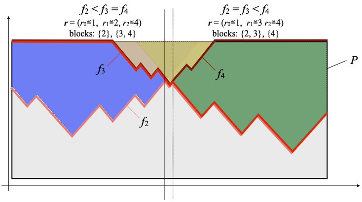
There is a zone on the left, consisting of those points z where f2 (z) < f3 (z) = f4 (z), namely of those points z that obey the partition r defined by r0≝1, r1≝2 and r2≝4, encoding the list of blocks {2} and {3, 4}. There is a zone on the right, consisting of those points z where f2 (z) = f3 (z) < f4 (z), namely of those points z that obey the partition r defined by r0≝1, r1≝3 and r2≝4, encoding the list of blocks {2, 3} and {4}. There is another zone in the middle, between the two dotted vertical lines, which consists of those points z where f2 (z) = f3 (z) = f4 (z), namely of those points z that obey the partition r defined by r0≝1, r1≝4, encoding the single block {2, 3, 4}. The zone of all points z that obey the final partition r0≝1, r1≝2, r3≝2 and r3≝4 is simply empty in our example: there are no points z such that f2 (z) < f3 (z) < f4 (z) here.
Lemma F. For almost every z ∈ [c, d] × [e, f], all the gradients ∇fr(z) exist, and if z obeys a partition r (written as above), then ∇fr0+1 (z) = … = ∇fr1 (z), ∇fr1+1 (z) = … = ∇fr2 (z), …, and ∇frm–1+1 (z) = … = ∇frm (z).
Proof. The first claim is because any finite union of sets of Lebesgue measure 0 is still a set of Lebesgue measure 0. For good measure, we will add the boundary of [c, d] × [e, f] to that union. This is still a set of Lebesgue measure 0, and this will allow us to make sure that z is in the interior of [c, d] × [e, f].
For the second claim, it suffices to look at any index r such that fr (z) = fr+1 (z), and to show that, necessarily, ∇fr (z) = ∇fr+1 (z). Since fr ≤ fr+1, the function fr+1–fr is non-negative. By assumption, it takes the value 0 at z, and its gradient exists at 0, and is equal to ∇fr+1 (z) – ∇fr (z). If the latter were non-zero, there would be a vector v such that |v|=1 and such that the directional derivative (∇fr+1 (z) – ∇fr (z)).v is non-zero. By replacing v by –v if necessary, we may assume that (∇fr+1 (z) – ∇fr (z)).v < 0. Since z is in the interior of [c, d] × [e, f], the points z+ε.v are still in [c, d] × [e, f] for all sufficiently small ε>0. Then fr+1–fr evaluated at z+ε.v is equal to ε(∇fr+1 (z) – ∇fr (z)).v + o(ε); this is a strictly negative value, which is impossible. Therefore ∇fr+1 (z) – ∇fr (z) = 0, so ∇fr (z) = ∇fr+1 (z). ☐
Let us return to our initial problem: showing that –∫P Qε(x) ∇ψ(x)T dx is in the matrix cone RC. By Lemma E, we can rewrite this value as:
y1 ∫P ∇ψ(x)T dx + ∑k=2N (yk – yk–1) . ∫P χUfk (x) ∇ψ(x)T dx.
The term ∫P ∇ψ(x)T dx is equal to 0. For example, its first coordinate is ∫–b–a B’[–b, –a] (x1) dx1 ∫cd B[c, d] (x2) dx2 ∫ef B[e, f] (x3) dx3, and ∫–b–a B’[–b, –a] (x1) dx1 = B[–b, –a] (–b) – B[–b, –a] (–a) = 0 – 0 = 0; the argument is similar for the second and third coordinates. Hence –∫P Qε(x) ∇ψ(x)T dx simplifies to:
∑k=2N (yk – yk–1) . ∫P χUfk (x) ∇ψ(x)T dx,
which is equal to:
∑k=2N (yk – yk–1) . ∫[c, d] × [e, f] ψ (fk (z), z) (1, –∇fk (z))T dz
by Lemma D. We split the integral in the latter formula into a finite sum over pairwise disjoint zones as follows. For every partitition r, let Zr be the collection of points z ∈ [c, d] × [e, f] that obey partition r. Let me call Zr the zone of the partition r. It is clear that the zones Zr partition the rectangle [c, d] × [e, f]. Also, writing r as the sequence of indices 1=r0 < r1 < … < rm=N, Zr is equal to {z ∈ [c, d] × [e, f] | fr0+1 (z) = … = fr1 (z) < fr1+1 (z) = … = fr2 (z) < … < frm–1+1 (z) = … = frm (z)}, and is therefore Borel measurable (we use that each fk is 1-Lipschitz, hence continuous, hence measurable; for any two real-valued measurable maps g and h, the set of points z such that g(z)=h(z) is measurable, since it is equal to ∩n ∈ N g–1 (]h (z)–1/2n, h (z)+1/2n[); therefore its complement is measurable, too).
Hence we can rewrite our latest formula for –∫P Qε(x) ∇ψ(x)T dx to:
∑r ∑k=2N (yk – yk–1) . ∫Zr ψ (fk (z), z) (1, –∇fk (z))T dz,
where r in the first sum ranges over all partitions of {2, …, N}. By Lemma F, for a fixed z in some set whose complement has Lebesgue measure 0, all the terms ∇fk (z) with k in the same block of r are equal. Writing r as 1=r0 < r1 < … < rm=N, this means that, given that k is in some block {rp–1+1, …, rp}, ∇fk (z) = ∇frp (z). Hence we can group terms in the inner summation over k blockwise, and we obtain that –∫P Qε(x) ∇ψ(x)T dx is equal to:
∑r=(1=r0 < r1 < … < rm=N) ∑p=1m (yrp – yrp–1) . ∫Zr ψ (frp (z), z) (1, –∇frp (z))T dz.
Here is the final miracle.
Lemma G. For every partitition r, say 1=r0 < r1 < … < rm=N, of {2, …, N}, for every p ∈ {1, …, m}, one of the following happens:
- frp (z) = –b, and then ψ (frp (z), z)= 0, or
- frp (z) = –a, and then ψ (frp (z), z) = 0, or
- yrp – yrp–1 is in C.
Before we prove this, let us look again at our example (reproduced below). In the left-hand zone, rp can be 2 or 4, and the Lemma says that y2 – y1 and y4 – y2 are in C, namely that y1 ≤C y2 and y2 ≤C y4. In the right-hand zone, rp can be 3 or 4, and the Lemma says that y3 – y1 and y4 – y3 are in C, namely that y1 ≤C y3 and y3 ≤C y4. In the middle zone (r0≝1, r1≝4), rp can only be 4, and the Lemma says that y4 – y1 is in C, namely that y1 ≤C y4. And indeed, all these inequalities between points of Im Qε do hold, as the rightmost part of the picture shows.
Proof. In case 1, and letting z be written as (x2, x3), ψ (frp (z), z) = B[–b, –a] (–b) B[c, d] (x2) B[e, f] (x3), which is equal to 0 since B[–b, –a] (–b) = 0. Case 2 is similar, since B[–b, –a] (–a) = 0.
We now assume that we are neither in case 1 nor in case 2. We have –b < frp–1+1 (z) = … = frp (z) < –a. Let s be such that –b < s < frp–1+1 (z). If p≥2, then additionally frp–1 (z) < frp–1+1 (z), and we additionally require that frp–1 (z) < s < frp–1+1 (z). Similarly, let t be such that frp (z) < t < –a, and t < frp+1 (z) if p<N.
- By definition of s, the point (s, z) is not in Qε–1(↑C yrp–1+1) ∪ … ∪ Qε–1(↑C yN), but is in Qε–1(↑C yrp–1) ∪ Qε–1(↑C yrp–1+1) ∪ … ∪ Qε–1(↑C yN) if p≥2. Hence Qε (s, z), which must be a point yk, can only be yrp–1.
- Similarly, by definition of t, the point Qε (t, z) is in Qε–1(↑C yrp) ∪ Qε–1(↑C yrp+1) ∪ … ∪ Qε–1(↑C yN), but is not in Qε–1(↑C yrp+1) ∪ … ∪ Qε–1(↑C yN) if r<N, so Qε (t, z) = yrp.
- But (t, z) – (s, z) = (t–s) e, where e is our old friend (1, 0, 0), which is in int(C) hence in C. Therefore (s, z) ≤C (t, z), and since Qε is monotonic, Qε (s, z) = yrp–1 ≤C Qε (t, z) = yrp. Hence we are in case 3, as promised. ☐
For each partition r, let Z’r be {z ∈ Zr | frp (z) ≠ –b, –a}. This is again a Borel measurable subset of [c, d] × [e, f], because this is Zr minus the union of the two closed subsets frp–1({–b}) and frp–1({–a}). Using Lemma G, items 1 and 2, ∫Zr–Z’r ψ (frp (z), z) (1, –∇frp (z))T dz is the integral the zero function, and is equal to 0. Hence ∫Zr ψ (frp (z), z) (1, –∇frp (z))T dz = ∫Z’r ψ (frp (z), z) (1, –∇frp (z))T dz; in other words, we may replace Zr by Z’r as domain of integration. Therefore, our latest formula for –∫P Qε(x) ∇ψ(x)T dx simplifies to the following, where we have replaced Zr by Z’r as domains of integration:
∑r=(1=r0 < r1 < … < rm=N), Z’r≠∅ ∑p=1m (yrp – yrp–1) . ∫Z‘r ψ (frp (z), z) (1, –∇frp (z))T dz,
and where we have also removed the partitions r such that Z’r is empty from the outer sum, since they contribute nothing to the summation. Then, the column vectors yrp – yrp–1 that remain in the above formula are all in C. This is by Lemma G, item 3.
Lemma H. The integral of any Lebesgue measurable function g : A → R3 over any domain A, such that g(z) ∈ C for almost all z ∈ A, is in C. As a consequence, for every partition r of {2, …, N}, written as 1=r0 < r1 < … < rm=N, for every p ∈ {1, …, m}, ∫Z‘r ψ (frp (z), z) (1, –∇frp (z)) dz is in C.
Proof. Let us write g(z) as the 3-tuple (g1 (z), g2 (z), g3 (z)). The integral of g is the triple (∫A g1 (z) dz, ∫A g2 (z) dz, ∫A g3 (z) dz). The Euclidean norm |(∫A g2 (z) dz, ∫A g3 (z) dz)| is less than or equal to the integral ∫A |(g2 (z), g3 (z))| dz of the Euclidean norms. This is a standard application of the Cauchy-Schwarz inequality, see this Math Stackexchange post if you are curious. For almost all z in A, g(z) is in C, so |(g2 (z), g3 (z))| ≤ g1 (z). Therefore |(∫A g2 (z) dz, ∫A g3 (z) dz)| ≤ ∫A g1 (z) dz, showing the first part of the Lemma.
For the second part, for almost every z in Z‘r, (1, –∇frp (z)) is in C by Lemma D. Since ψ (frp (z), z) ≥ 0 and C is a cone, ψ (frp (z), z) (1, –∇frp (z)) is also in C. We take the latter to be the function g (z) of z, to which we apply the first part of the Lemma. ☐
Summing up, –∫P Qε(x) ∇ψ(x)T dx is a finite sum, over all partitions r of {2, …, N}, written as 1=r0 < r1 < … < rm=N, such that Z’r is non-empty, and over all indices p ∈ {1, …, m}, of terms of the form v wT, where v ≝ yrp – yrp–1 is in C and w ≝ ∫Z‘r ψ (frp (z), z) (1, –∇frp (z)) dz in in C by Lemma H.
It follows that –∫P Qε(x) ∇ψ(x)T dx is in the matrix cone RC. Phew! Point 1 done.
There remains only two things to prove, but they are easy.
–∫P Qε(x) ∇ψ(x)T dx tends to the 3 × 3 identity matrix I3
By Lemma 3.1 [1] (which we have reproved earlier in this post), Qε(x) tends uniformy to x on P as ε tends to 0. Hence –∫P Qε(x) ∇ψ(x)T dx tends to –∫P x ∇ψ(x)T dx. If you know about Lebesgue’s dominated convergence theorem, this is easy. But you don’t even need to know about it. For every ε>0, Qε(x) is in the closed interval [x–ε.e, x], so ∫P Qε(x) ∇ψ(x)T dx lies between ∫P x ∇ψ(x)T dx – ε.e ∫P ∇ψ(x)T dx and ∫P x ∇ψ(x)T dx, and the error term ε.e ∫P ∇ψ(x)T dx tends to the zero matrix as ε tends to infinity.
It remains to show that –∫P x ∇ψ(x)T dx = I3. Since I have taken ψ of a very specific form, this is easy. Chen, Kou and Lyu use the Gauss-Green formula, but we will only need to do some integration by parts on the real line. Let me recall that ψ(x) = B[–b, –a] (x1) B[c, d] (x2) B[e, f] (x3).
For all indices i, j among {1, 2, 3}, the (i, j) entry of the matrix –∫P x ∇ψ(x)T dx is –∫P xi ∂ψ (x)/∂xj dx.
- When i≠j, say i ≝ 1 and j ≝ 2 (all other cases are similar), this is equal to the product of the three integrals ∫–b–a x1 B[–b, –a] (x1) dx1, ∫cd B’[c, d] (x2) dx2, and ∫ef B[e, f] (x3) dx3. But ∫cd B’[c, d] (x2) dx2 = B[c, d] (d) – B[c, d] (c) = 0 – 0 = 0.
- When i=j, say i ≝ 1 and j ≝ 1 (the other two cases are similar), then –∫P xi ∂ψ (x)/∂xj dx is equal to the product of the three integrals ∫–b–a x1 B’[–b, –a] (x1) dx1, ∫cd B[c, d] (x2) dx2 and ∫ef B[e, f] (x3) dx3. The first one is equal to [x1 B[–b, –a] (x1)]–b–a – ∫–b–a 1 . B[–b, –a] (x1) dx1, by using integration by parts; now [x1 B[–b, –a] (x1)]–b–a = –a B[–b, –a] (–a) + b B[–b, –a] (–b) = 0 and ∫–b–a 1 . B[–b, –a] (x1) dx1 = ∫–b–a B[–b, –a] (x1) dx1 = 1. We also recall that ∫cd B[c, d] (x2) dx2 and ∫ef B[e, f] (x3) are equal to 1, so –∫P xi ∂ψ (x)/∂xj dx = 1.
It follows that –∫P x ∇ψ(x)T dx is the identity matrix I3.
By Proposition 4.1 [1] (which we have reproved earlier in this post), RC is closed. Since the identity matrix I3 is a limit of elements –∫P Qε(x) ∇ψ(x)T dx of RC, I3 is in RC. It remains to see that this is impossible.
I3 is not in RC
In order to show that I3 is not in RC, we will find an invariant, namely a property that is true of all elements of RC, and which fails for I3. This invariant will be in a form of a linear map Λ that only takes non-negative values on RC.
Let J be the diagonal 3 × 3 matrix with entries 1, –1 and –1, namely. This is a well-known object: J is the matrix representation of the Minkowski metric in 2+1 dimensions.
Let me write tr(A) for the trace of a 3 × 3 matrix A. There is a linear map Λ : Mat (3, 3) → R defined by Λ(A) ≝ tr(JA). For all elements v and w of C, writing v as (v1 v2 v3)T and w as (w1 w2 w3)T, v wT is the matrix , so J v wT is the matrix . Therefore Λ (v wT) = v1 w1 – v2 w2 – v3 w3.
We observe that v2 w2 + v3 w3 is the scalar product of (v2 v3) with (w2 w3). By the Cauchy-Schwarz inequality, it is less than or equal to the product of the norms |(v2 v3)| and |(w2 w3)| of the two vectors. By definition of C, v1 ≥ |(v2 v3)| and w1 ≥ |(w2 w3)|, so v1 w1 ≥ |(v2 v3)| . |(w2 w3)| ≥ v2 w2 + v3 w3, and therefore Λ (v wT) ≥ 0.
If A is any element ∑i=1m ai . vi wiT of RC, where each ai is non-negative and vi, wi are in C, then:
Λ(A) = ∑i=1m ai Λ (vi wiT) ≥ 0.
However, Λ (I3) = 1 – 1 – 1 = –1. Therefore I3 is not in RC. This completes the proof: Disc is not an RB-domain, and therefore FS≠RB.
A final note
Zhenchao Lyu tells me that Yuxu Chen, Hui Kou and himself have also solved a big part of another outstanding problem in domain theory: whether the probabilistic powerdomain of an RB-domain is an RB-domain. The answer is no [4]. In fact, they show much more: the finite posets X whose probabilistic powerdomain (precisely, whose dcpos of subprobability valuations) is an RB-domain are exactly the finite trees. Amazing.
- Yuxu Chen, Hui Kou, and Zhenchao Lyu. FS-domains are not always RB-domains. arXiv report 2607.00568v2, July 04th, 2026.
- Achim Jung. The classification of continuous domains. Proceedings of the 5th Annual IEEE Symposium on Logics in Computer Science (LICS’90), 1990, pages 35-40.
- Lawrence C. Evans. Measure theory and fine properties of functions. Chapman and Hall/CRC, 2025.
- Yuxu Chen, Hui Kou, and Zhenchao Lyu. Characterizing finite posets whose probabilistic powerdomains are RB-domains. arXiv report 2607.02231, July 2nd, 2026.

— Jean Goubault-Larrecq (July 14th, 2026)