Let us analyze a dcpo proposed in 1993 by Peter Knijnenburg [1, Example 6.1]. The original purpose of that dcpo was to show an example of a dcpo such that the Egli-Milner and the topological Egli-Milner orderings differ on its space of lenses. (If you don’t understand, don’t worry: if I ever speak about that, I will explain everyting that is needed first.) It is a funny little dcpo that serves as a counterexample for several questions.
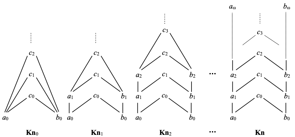
Here is the dcpo he proposes:

Let me call this poset Kn. It contains elements a0 < a1 < … < an < … and their supremum aω, a similar chain of elements b0 < b1 < … < bn < … and their supremum bω, and all the ais and the bjs being pairwise incomparable; and it contains elements c0, c1, …, cn, … organized in such a way that those form an antichain (no two elements ci are comparable) and that each ci is located right above ai and bi.
Formally, the ordering on Kn is given by: am ≤ an, bm ≤ bn, am ≤ cn, bm ≤ cn are all equivalent to m≤n; all other pairs of elements are incomparable. In particular, every element cn is maximal in this ordering.
Achim Jung also came up with something similar in his PhD thesis, defended a few years previously: his example of an algebraic dcpo “in which the base has property m but the dcpo itself doesn’t” [5, Figure 1.8], contains a copy of Kn in its lower layer.
Basic properties of Kn
Lemma A. Kn is a dcpo.
Proof. Given a directed family D, either D is trivial (contains a largest element x) and then it is easy to see that x is its supremum, or D is non-trivial. If D is non-trivial, then it cannot contain any maximal element of Kn, which would then be the largest element of D, since D is directed; and then D would be trivial. Hence D cannot contain aω, bω, and cannot contain any cn either. If D contains some am and some bn, then it must contain an upper bound of those two, and that can only be an element of the form ck; but we have just seen that such elements cannot be in D. Therefore D is entirely contain in what I will call the a-column {an | n ∈ N} or in the b-column {bn | n ∈ N}. Since D is non-trivial, D must then be a collection of elements an in the a-column with n unbounded or a collection of elements bn in the b-column with n unbounded. In the first case, sup D=aω, and in the second case, sup D=bω. ☐
Kn is, in some sense, a pretty nice dcpo. I will let you prove the following by yourselves. You only need to consider non-trivial directed families, as in the proof of Lemma A.
Lemma B. Kn is an algebraic dcpo, whose finite elements are all its elements except aω and bω.
In particular, with its Scott topology, Kn is a locally compact, sober space. It is even compact, since it is equal to the upward closure of the finite set {a0, b0}.
Lemma C. The intersection of the two compact saturated subsets ↑a0 and ↑b0 is the non-compact set {c0, c1, …, cn, …}. Hence Kn is not coherent.
Proof. For each n ∈ N, {cn} is upwards-closed since cn is maximal in Kn. Then {cn}=↑cn. But cn is a finite element of Kn, by Lemma B, so ↑cn is Scott-open. In order to see that {c0, c1, …, cn, …} is not compact, it suffices to observe that the one-element sets {cn} with n ∈ N are all Scott-open, as we have just seen, and form an open cover that simply has no proper subcover, and in particular no finite subcover. ☐
Let us turn to weak Hausdorffness [3, Lemma 6.6]. A space X is weakly Hausdorff if and only if:
- for any two points x and y in X,
- for every open neighborhood W of ↑x ∩ ↑y,
- there is an open neighborhood U of x and there is an open neighborhood V of y
- such that U ∩ V ⊆ W.
The notion of weak Hausdorffness is an interesting one, I think, and I have given a few results on the notion in the November 2022 post.
Lemma D. Kn is not weakly Hausdorff.
Proof. We take x ≝ aω, y ≝ bω, and the empty set for W. It is clear that ↑aω ∩ ↑bω is included in W: it is empty. Let us assume that we could find an open neighborhood U of aω and an open neighborhood V of aω such that U ∩ V ⊆ W. Since aω is the supremum of the a-column {am | m ∈ N}, some am must be in U. Similarly, some bn must be in V. Then cmax(m,n) is above am and bn, and must therefore be in U ∩ V. This is impossible since U ∩ V is included in W, that is, since U ∩ V is empty. ☐
Downward closures of lenses
A lens L in a topological space X is a non-empty intersection Q ∩ C of a compact saturated subset Q and of a closed subset C of X. The notion arises naturally in the study of the Plotkin powerdomain of X.
Every lens is compact, since it is the intersection of a compact set with a closed set (Corollary 4.4.10 in the book). It is also patch-closed, namely closed in the patch topology on X (see Definition 9.1.26 in the book), because the patch topology is by definition the coarsest topology that makes every compact saturated subset of X and every closed subset X (patch-)closed. A lens L is also order-convex, in the sense that for all points x≤y≤z, if x and z are in L, then y is in L: indeed, if x is in L (=Q ∩ C), then x is in Q, and since Q is upwards-closed, y is in Q; and if z is in L, then z is in C, and since C is downwards-closed, y is in C; being both in Q and in C, y is in L.
Lenses are at their best when X is stably compact. Let me explain why, then let me explain why we still get a lot on weakly Hausdorff spaces, and then how Kn shows that the assumptions we will make are needed.
We start with something that is always true, whatever assumptions we make on X.
Lemma E. Given a lens L on a topological space X, there is a canonical way of writing L as Q ∩ C with Q compact saturated and C closed, which consists in defining Q as ↑L and C as the closure cl(L). By “canonical”, we mean that among the possible pairs of a compact saturated set and a closed set whose intersection is equal to L, (↑L, cl(L)) is the smallest one in the product ordering ⊆ × ⊆.
Proof. Let us write L as Q0 ∩ C0, where Q0 is compact saturated and C0 is closed. Since L is compact, its upward closure Q ≝ ↑L is compact, too (Proposition 4.4.14 in the book), and is saturated (=upwards-closed) by definition. The closure cl(L) is trivially closed. It remains to show that L = Q ∩ C.
We note that Q ⊆ Q0. Indeed, for every point x in Q, there is a point y in L such that y≤x, by definition of Q, and then y must be in Q0, since L = Q0 ∩ C0. Since Q0 is saturated, x must be in Q0.
We also note that C ⊆ C0. This is because L ⊆ C0, and since C0 is closed, the closure of L, which is C, must also be included in C0.
Those two remarks show the canonicality statement. They also imply that Q ∩ C ⊆ Q0 ∩ C0 = L. The reverse inclusion is easy: for every point x in L, x is trivially both in ↑L = Q and in cl(L) = C, hence in Q ∩ C. ☐
Now there is an asymmetry here: for Q, we take the upward closure of L, while for C, we take the closure, not the downward closure of L. This difficulty permeates the whole theory of lenses. When X is stably compact, this does not matter, as the following lemma explains.
Lemma F. For every patch-closed subset K of a stably compact space X, in particular for every lens, ↓K is closed in X; in particular, ↓K=cl(K).
Proof. The proof is pretty short once we know enough about the tight connection between stably compact spaces and compact pospaces (Section 9.1 of the book). Let me recall a bit of it. Given that X is stably compact, its de Groot dual Xd has the same points as X, but its open subsets are the complements of the compact saturated subsets of X; equivalently, the closed subsets of Xd are the compact saturated subsets of X. The specialization ordering of Xd is the opposite ≥ of the specialization ordering ≤ of X. The patch topology on X is generated by the open subsets and the complements of the compact saturated subsets of X. We write Xpatch for X with the patch topology. If X is stably compact, then Xpatch is compact Hausdorff, and the original specialization ordering ≤ on X is closed, meaning that its graph (≤) is a closed subset of Xpatch × Xpatch. Additionally, the open subsets of X are exactly the upwards-closed (with respect to ≤) open subsets of Xpatch; in other words, the closed subsets of X are exactly the downwards-closed, closed subsets of Xpatch. By this remark, we will reach our goal to prove that ↓K is closed if we can prove that ↓K is closed in Xpatch.
Since K is patch-closed, namely closed in Xpatch, and since Xpatch is compact, K is compact in Xpatch. As a product of two compact spaces, Xpatch × Xpatch is compact. The graph (≤) is closed in the latter, and Xpatch × K is compact, as a product of two compact subsets of Xpatch. Therefore their intersection (≤) ⋂ (Xpatch × K) is compact in Xpatch × Xpatch. Writing π1 for the map (x, y) ↦ x from Xpatch × Xpatch onto Xpatch, we see that π1 is continuous (by definition of the product topology on Xpatch × Xpatch), so the image π1[(≤) ⋂ (Xpatch × K)] is compact in Xpatch. But π1[(≤) ⋂ (Xpatch × K)] = {x | for some y in Xpatch, x≤y and y ∈ K} = ↓K. We have just shown that ↓K is compact in Xpatch. Since Xpatch is Hausdorff, ↓K is closed in Xpatch. It is downwards-closed, so it is closed in X.
This proves the first part of the claim, that ↓K is closed in X. Since cl(K) is downwards-closed and contains K, it contains ↓K. Since ↓K is closed, as we have just seen, and contains K, it contains its closure cl(K). Therefore ↓K = cl(K). ☐
Lemma F applies to every patch-closed subset of a stably compact space, not just the lenses. If we are only interested in lenses, we only need to assume that X is weakly Hausdorff [2, Theorem 6.4]. Let me recall that every stably compact space is weakly Hausdorff (see the November, 2022 post, where we even showed that every stably locally compact space is weakly Hausdorff; the result is due to Keimel and Lawson [3, Lemma 8.1]).
The proof is elementary, contrarily to the proof we just gave of Lemma F. We will only need the following equivalent characterization of weakly Hausdorff spaces; this was proved in the appendix of the November, 2022 post, and is also due to Keimel and Lawson [3, Lemma 6.6].
Fact G. A space X is weakly Hausdorff if and only if for any two compact saturated subsets Q1 and Q2 in X, for every open neighborhood W of Q1 ∩ Q2, there is an open neighborhood U of Q1 and there is an open neighborhood V of Q2 such that U ∩ V ⊆ W.
Lemma H. For every lens L in a weakly Hausdorff space, ↓L is closed in X; in particular, ↓L=cl(L).
Proof. The second part follows from the first one, as in the proof of Lemma F.
Let us write L as Q ∩ C where Q is compact saturated and C is closed. In order to show that ↓L is closed, we consider any point x lying outside of ↓L, and we will find an open neighborhood of x that does not intersect ↓L; this will show that the complement of ↓L is open, hence that ↓L is closed.
Since x ∉ ↓L by assumption, the upward closure ↑x does not intersect L: if it intersected it, say at some point y, then we would have x≤y and y ∈ L, hence x ∈ ↓L. That ↑x does not intersect L rewrites as ↑x ∩ (Q ∩ C) = ∅, equivalently as (↑x ∩ Q) ∩ C = ∅, equivalently as ↑x ∩ Q ⊆ W, where W is the complement of C.
W is open, ↑x and Q are compact saturated. By Fact G, there is an open neighborhood U of ↑x and there is an open neighborhood V of Q such that U ∩ V ⊆ W. U is our desired neighborhood of x: it remains to show that it does not intersect ↓L. Let us imagine it did, and let y ∈ L be such that x ≤ y. Then y ∈ U, since ↑x ⊆ U. Also, y is in L, hence in Q, hence in V. Therefore y is in U ∩ V, hence in W. In other words, y is not in C, since W is the complement of C, and that is impossible since y is in L = Q ∩ C. ☐
At this point, one may wonder whether ↓L=cl(L) for every lens L of any topological space whatsoever. Knijnenburg’s dcpo Kn provides us with the desired counterexample.
Counterexample I. In Kn, L ≝ {c0, c1, …, cn, …} ∪ {bω} is a lens but ↓L is not closed, equivalently ↓L≠cl(L). Indeed, ↓L = Kn – {aω} and cl(L) = Kn.
In order to show this, we will have to verify that L is a lens. But let us compute ↓L and cl(L) as a first step. This is easier to see on a picture. Below, I have drawn L in blue, and ↓L in green. Only aω is not in ↓L. In order to show that cl(L) is the whole of Kn, we note that cl(L) is downwards-closed and contains L, hence also ↓L; then, that since cl(L) is closed and we now know that it contains the sequence {a0, a1, …, an, …} (in ↓L), it must also contain the supremum of that sequence, which is aω.

It remains to show that L is a lens. We profit from Lemma E: if E is a lens, then we can write it as the intersection of the set ↑L, which should be compact saturated, and of the closed set cl(L).
Let Q ≝ ↑L. Since L consists of maximal elements of Kn, Q is in fact equal to L. It remains to see that Q is compact. Let (Ui)i ∈ I be an open cover of Q. The element bω is in Ui for some i ∈ I. Since Ui is Scott-open and bω is the supremum of {b0, b1, …, bn, …}, Ui must contain every bn for n large enough, say n≥n0. But cn ≥ bn and Ui is upwards-closed, so Ui contains cn for every n≥n0. The remaining finitely many elements c0, c1, …, cn–1 are covered by finitely many open sets Uj. Together with Ui, they form an open cover of L (=Q).
Now Q = L, C ≝ cl(L) is equal to the whole of Kn, so Q ∩ C = L. ☐
The Plotkin powerdomain
I have talked a bit about the Plotkin powerdomain of a space X in the March 2021 post. There are several inequivalent definitions in general, but a popular one is to take the space of all lenses on X, with a certain topology. Let me call PX this set of all lenses.
One of the most natural topologies is the Vietoris topology, which has a subbase consisting of open sets of the form ☐U ≝ {L ∈ PX | L ⊆ U} or ♢U ≝ {L ∈ PX | L intersects U}, where U ranges over the open subsets of X.
With the Vietoris topology, PX is a space whose specialization (pre)ordering is the topological Egli-Milner ordering ⊑TEM, defined by L ⊑TEM L’ if and only if ↑L ⊇ ↑L’ and cl(L) ⊆ cl(L’).
Let us prove this right away. If L is below L’ in the specialization preordering of the Vietoris topology, then for every open subset U of X, if L ∈ ☐U then L’ ∈ ☐U. In other words, L’ is in intersection of all the open neighborhoods of L. But that intersection is the saturation ↑L of L (Proposition 4.2.9 in the book). Hence L’ ⊆ ↑L, equivalently ↑L ⊇ ↑L’. Similarly, for every open subset U of X, if L ∈ ♢U then L’ ∈ ♢U. Letting U be the complement of cl(L’), it is wrong that L’ ∈ ♢U, so, by contraposition, L is not in ♢U, namely L is included in the complement of U, which is cl(L’). From L ⊆ cl(L’), we deduce that cl(L) ⊆ cl(L’). Therefore L ⊑TEM L’. Conversely, let us assume that L ⊑TEM L’. In order to show that L is below L’ in the specialization preordering of the Vietoris topology, it suffices to show that for every open subset U of X, if L ∈ ☐U then L’ ∈ ☐U and if L ∈ ♢U then L’ ∈ ♢U. If L ∈ ☐U, then L is included in U, and therefore ↑L is included in U, since U is upwards-closed. From L ⊑TEM L’, we obtain that ↑L ⊇ ↑L’, so ↑L’ is included in U; whence L’ ∈ ☐U. If L ∈ ♢U, then L intersects U, hence the larger set cl(L) also intersects U. From L ⊑TEM L’, we obtain that cl(L) ⊆ cl(L’), so cl(L’) intersects U, hence L’ also intersects U. Therefore L’ ∈ ♢U.
By the way, ⊑TEM is a partial ordering, not just a preordering, and therefore PX is T0. Indeed, if L ⊑TEM L’ and L’ ⊑TEM L, then ↑L = ↑L’ and cl(L) = cl(L’). By Lemma E, L = ↑L ⋂ cl(L) and L’ = ↑L’ ⋂ cl(L’), so L = L’.
In domain theory, another ordering is usually preferred, probably because it is easier to handle. This is the Egli-Milner ordering ⊑EM, defined by L ⊑EM L’ if and only if ↑L ⊇ ↑L’ and ↓L ⊆ ↓L’. Also, on aesthetic grounds, its definition is more symmetrical.
The good news is that, if X is weakly Hausdorff, then ⊑EM and ⊑TEM are the same ordering! This follows directly from Lemma H. Knijnenburg had produced the dcpo Kn in order to show that the two orderings differ on general dcpos. Let us check that.
Counterexample J. On P(Kn), ⊑EM and ⊑TEM differ: L ≝ {c0, c1, …, cn, …} ∪ {bω} and the whole of Kn are lenses, and Kn ⊑TEM L but Kn ⋢EM L.
Indeed, we recall from Countexample I that L is a lens. Kn itself is a lens, since it is compact (being the upward closure of finitely many—two—points) and closed; so Kn = Q ∩ C with Q and C both defined as Kn. We have ↑Kn ⊇ ↑L, trivially. We also have cl(Kn) ⊆ cl(L), because cl(Kn)=Kn (trivially) and cl(L) = Kn, as we have seen in Couterexample I. But ↓Kn ⊊ ↓L because aω is in ↓Kn=Kn and not in ↓L = Kn – {aω} (see Counterexample I, again).
Projective limits
Knijnenburg’s dcpo also provides an easy way to show that projective limits of weakly Hausdorff spaces fail to be weakly Hausdorff in general. That is the case even for projective limits of projective systems (pmn : Xn → Xm)m≤n in N with countably many weakly Hausdorff spaces Xn that are also sober, and where the bonding maps pmn are not just continuous but are even projections, meaning that they have matching embeddings emn : Xm → Xn with the property that pmn o emn = id and emn o pmn ≤ id.
For every n ∈ N, let Knn be the subposet of Kn consisting of a0, a1, …, an, of b0, b1, …, bn, and of c0, c1, …, cn, cn+1, … (all the constants ci). Here is a depiction of the first spaces Knn. We will show that, with pretty obvious definitions of pmn (and emn), these spaces fit into a projective system whose projective limit is Kn, shown on the right.
We equip each Knn with its Scott topology. But wait: there is no non-trivial directed subset in Knn. Hence Knn is a dcpo, and all of its elements are finite, for a trivial reason. The Scott topology is then generated by the open subsets ↑x, where x ranges over the points. But the topology generated this way consists exactly of the upwards-closed subsets of Knn: the topology of Knn is the Alexandroff topology. In the November 2022 post, we have observed that every space with an Alexandroff topology is weakly Hausdorff. Therefore every Knn is weakly Hausdorff. Every Knn is also an algebraic dcpo (in which every point is finite), and is therefore sober.
For every n ∈ N, let pn : Kn → Knn map every ak to amin(k,n), every bk to bmin(k,n), and every ck to itself. This is a Scott-continuous map. In order to see this, we first note that pn is monotonic; then it suffices to show that pn preserves suprema of non-trivial directed subsets. Near the beginning of this post, we had seen that the only non-trivial directed subsets of Kn are those that are included in the a-column, with elements ak with arbitrarily large values of k, and those that are included in the b-column, with elements bk with arbitrarily large values of k. The supremum of those of the first kind is aω, which is mapped to amin(ω,n) = an by pn, and that is also the supremum of the elements p(ak): as k is unbounded, eventually k exceeds n, and then p(ak) = amin(k,n) = an.
For every pair m≤n of natural numbers, let pmn : Knn → Knm be the restriction of pm to the subposet Knn of Kn. This is a Scott-continuous map simply because it is monotonic and there is no non-trivial directed subset of Knn at all. Those maps organize into a projective system, since pmm = id and plm o pmn = pln for all l≤m≤n.
The corresponding embeddings emn : Knm → Knn (for all m≤n) are simply the inclusions. They are Scott-continuous because they are monotonic and there is no non-trivial directed subset of Knm. The facts that pmn o emn = id and emn o pmn ≤ id are obvious: the first one means that if k≤n, then amin(k,n) = ak and bmin(k,n) = bk, and the second one means that for every natural number k, amin(k,n) ≤ ak and bmin(k,n) ≤ bk.
I claim that Kn, with the maps pn : Kn → Knn, is a projective limit of (pmn : Knn → Knm)m≤n in N. It suffices to verify the universal property of projective limits directly. Let us imagine we have another space X with continuous maps qn : X → Knn for each natural number n, such that for all m≤n, pmn o qn = qm. We wish to show that there is a unique continuous map f : X → Kn such that for every n ∈ N, pn o f = qn.
- If f exists, then it must map every x ∈ X to some element ak, bk or ck. In the ck case, p0(ck)=ck, so q0(x)=p0(f(x))=f(x), and this determines f(x) uniquely as q0(x). In the ak case, either k is finite or not. If k is finite, then we can pick n≥k, so that pn(ak)=ak, whence qn(x)=pn(f(x))=f(x), and this determines f(x) uniquely as qn(x) (for any n large enough). If k=ω, then for every n ∈ N, qn(x)=pn(f(x))=an, and this determines f(x) uniquely as supn ∈ N qn(x). Similarly in the bk case. Summarizing and simplifying, in all cases, f(x) must be equal to supn ∈ N qn(x).
- In order to show existence, for every x ∈ X, let us define f(x) as supn ∈ N qn(x), where the supremum is taken in Kn. For all m≤n, pmn o qn = qm, so pmn(qn(x)) = qm(x). In Kn, pmn(qn(x)) ≤ qn(x), so qm(x) ≤ qn(x). This shows that the supremum defining f(x) is the supremum of an ascending chain, which is well-defined since Kn is a dcpo.
- We have defined f as the pointwise supremum of a directed family of Scott-continuous maps (technically, the maps en o qn, where en is the inclusion of Knn in Kn), hence f is itself Scott-continuous.
- For every m ∈ N, we wish to show that pm o f = qm. For every x ∈ X, pm(f(x)) = pm(supn ∈ N qn(x)) = supn ∈ N pm(qn(x)) (since pm is Scott-continuous) = supn≥m pm(qn(x)) (since the family of natural numbers m larger than or equal to n is cofinal in N). But, for n≥m, pm(qn(x)) = pmn(qn(x)) (since pmn is the restriction of pm to Knn, in which qn takes its values) = qm(x) (since pmn o qn = qm). Therefore pm(f(x)) = supn≥m qm(x) = qm(x).
All this shows the following.
Counterexample K. Kn, with the maps pn : Kn → Knn, is a projective limit of (pmn : Knn → Knm)m≤n in N. The spaces Knn are weakly Hausdorff (and even have the Alexandroff topology of their ordering), sober, but Kn is not weakly Hausdorff.
One may wonder about coherence. The spaces Knn are not coherent, because the intersection of the compact saturated sets ↑a0 and ↑b0 is the subset {c0, c1, …, cn, …}, which is not compact: as in Lemma C, the open cover consisting of the one-element sets {cn} has no proper subcover, hence no finite subcover. I will leave the following as an exercise.
Exercise L. Define variants Kn‘n of the spaces Knn as follows: Kn‘n has the same points as Knn, and the same ordering, except that additionally we declare that cn≤cn+1≤… The points c0, c1, …, cn remain pairwise incomparable. Show that:
- (pmn : Kn‘n → Kn‘m)m≤n in N is also a projective system of weakly Hausdorff spaces;
- this time, the spaces Kn‘n are coherent (in fact even Noetherian, see Section 9.7 of the book), but not sober (not even monotone convergence spaces—in fact there is an ascending chain that does not have a supremum at all);
- Kn, with the maps pn : Kn → Kn‘n, is a projective limit of (pmn : Kn‘n → Kn‘m)m≤n in N.
- Therefore projective limits of weakly Hausdorff, coherent spaces fail to be weakly Hausdorff, and fail to be coherent, in general.
Oh, but what about projective limits of weakly Hausdorff, coherent sober spaces? Well, it turns out that they are always weakly Hausdorff, coherent and sober, equivalently locally strongly sober, see [4, Theorem 5.1]. Please allow me to omit the proof here, and let me just say that it rests on consequences of Steenrod’s theorem, which I covered in the September 2018 and October 2018 posts.
A final note
I have some basic notions of Dutch, and in particular I am pretty confident I know how “Knijnenburg” is pronounced in Dutch. This is pretty hard to explain in English. I have tried to find an Internet site that would explain it, but the first site I came to proposed US or UK pronunciations sounding like “Ninnenberg”. You cannot be farther away from the actual Dutch pronunciation. First, the initial K is pronounced. Second, the “ij” in the middle is pronounced somehow like “ay”, like in clay or gray (with some regional variations which sound like “eye” or a mix between those two). Third, the “n” before “burg” is essentially silent: think of pronouncing the English article “an” and then stopping right before uttering the “n”, making it an English schwa. (Correction, December 19, 2025: it seems that this “n” is pronounced, after all, except possibly in some regions.) Fourth, the ending “burg” is probably too hard to even try to pronounce if you are not trained into it (it is something like “burkh”, where “kh” is like the final “ch” in the German “ach”, although it can be softer and almost like the “ch” in German “ich”, depending on your form of Dutch). Maybe the closest you can do in English is to say “Cnaynaberg” (or “Cnaynenberg”), with the first syllable stressed, and ignoring the difficulty with the final consonants. But please, no “Ninnenberg”.
- Peter Knijnenburg. Algebraic Domains, Chain Completion and the Plotkin Powerdomain Construction. Utrecht University technical report RUU-CS-93-03, January 1993.
- Jean Goubault-Larrecq. On weakly Hausdorff spaces and locally strongly sober spaces. arXiv report 2211.10400, November 21st, 2022. Published in Topology Proceedings 62, 117–131, 2023.
- Klaus Keimel and Jimmie Lawson. Measure extension theorems for T0-spaces. Topology and its Applications, 149(1–3), 57–83, 2005.
- Jean Goubault-Larrecq. A few projective classes of (non-Hausdorff) topological spaces. Topology and its Applications 356:109009, Oct. 2024. See also https://arxiv.org/abs/2404.18614.
- Achim Jung. Cartesian closed categories of domains. PhD thesis, Technische Hochschule Darmstadt, 1988.

— Jean Goubault-Larrecq (November 20th, 2025)